4.2.1.7. ESA CCI Toolbox Vector Data Cube Access

The ESA CCI Toolbox also provides access to data that is provided in the form of vector data cubes. These can be thought of as a hybrid between data cubes and vector data. It is a data cube where the spatial locations are not identified through a structured grid, but distinct geometries.

To run this Notebook, make sure the ESA CCI Toolbox is setup correctly.

For this notebook, we start as before, by opening the standard esa-cci data store.

from xcube.core.store import new_data_store

cci_store = new_data_store('esa-cci')

The data in question are ICESHEETS and SEALEVEL datasets. We can find the vector data cubes by specifying their data type.

descriptors = cci_store.search_data(
    data_type="vectordatacube",
)
[descriptor.data_id for descriptor in descriptors]

['esacci.ICESHEETS.yr.Unspecified.GMB.GRACE-instrument.GRACE.UNSPECIFIED.1-2.greenland_gmb_mass_trends',
 'esacci.ICESHEETS.yr.Unspecified.GMB.GRACE-instrument.GRACE.UNSPECIFIED.1-3.greenland_gmb_mass_trends',
 'esacci.ICESHEETS.yr.Unspecified.GMB.GRACE-instrument.GRACE.UNSPECIFIED.1-4.greenland_gmb_mass_trends',
 'esacci.ICESHEETS.yr.Unspecified.GMB.GRACE-instrument.GRACE.UNSPECIFIED.1-5.greenland_gmb_mass_trends',
 'esacci.SEALEVEL.mon.IND.MSLTR.multi-sensor.multi-platform.MERGED.2-2.ASA',
 'esacci.SEALEVEL.mon.IND.MSLTR.multi-sensor.multi-platform.MERGED.2-2.BENGUELA',
 'esacci.SEALEVEL.mon.IND.MSLTR.multi-sensor.multi-platform.MERGED.2-2.CARIBBEAN',
 'esacci.SEALEVEL.mon.IND.MSLTR.multi-sensor.multi-platform.MERGED.2-2.GULFSTREAM',
 'esacci.SEALEVEL.mon.IND.MSLTR.multi-sensor.multi-platform.MERGED.2-2.HUMBOLDT',
 'esacci.SEALEVEL.mon.IND.MSLTR.multi-sensor.multi-platform.MERGED.2-2.MED_SEA',
 'esacci.SEALEVEL.mon.IND.MSLTR.multi-sensor.multi-platform.MERGED.2-2.NE_ATL',
 'esacci.SEALEVEL.mon.IND.MSLTR.multi-sensor.multi-platform.MERGED.2-2.N_INDIAN',
 'esacci.SEALEVEL.mon.IND.MSLTR.multi-sensor.multi-platform.MERGED.2-2.SE_AFRICA',
 'esacci.SEALEVEL.mon.IND.MSLTR.multi-sensor.multi-platform.MERGED.2-2.SE_ASIA',
 'esacci.SEALEVEL.mon.IND.MSLTR.multi-sensor.multi-platform.MERGED.2-2.S_AUSTRALIA',
 'esacci.SEALEVEL.mon.IND.MSLTR.multi-sensor.multi-platform.MERGED.2-2.WAFRICA',
 'esacci.SEALEVEL.mon.IND.MSLTR.multi-sensor.multi-platform.MERGED.2-2.r1']

We have a closer look at the first sea level dataset.

descriptors[4]

<xcube_cci.vdcaccess.VectorDataCubeDescriptor at 0x7c12e3a03a80>

Now, we can open the dataset to see what the vector data cube looks like.

sl_ds = cci_store.open_data(
    "esacci.SEALEVEL.mon.IND.MSLTR.multi-sensor.multi-platform.MERGED.2-2.ASA"
)

sl_ds

<xarray.Dataset> Size: 2MB
Dimensions:                (nbpoints: 2066, nbmonth: 216, bnds: 2)
Coordinates:
  * geometry               (nbpoints) object 17kB POINT (-67.60308074951172 -...
  * nbmonth                (nbmonth) datetime64[ns] 2kB 2002-01-16T12:00:00 ....
    nbmonth_bnds           (nbmonth, bnds) datetime64[ns] 3kB dask.array<chunksize=(216, 2), meta=np.ndarray>
Dimensions without coordinates: nbpoints, bnds
Data variables:
    distance_to_coast      (nbpoints) float32 8kB dask.array<chunksize=(50,), meta=np.ndarray>
    lat                    float64 8B ...
    local_sla_trend        (nbpoints) float32 8kB dask.array<chunksize=(50,), meta=np.ndarray>
    local_sla_trend_error  (nbpoints) float32 8kB dask.array<chunksize=(50,), meta=np.ndarray>
    lon                    float64 8B ...
    sla                    (nbpoints, nbmonth) float32 2MB dask.array<chunksize=(50, 216), meta=np.ndarray>
Indexes:
    geometry  GeometryIndex (crs=None)
Attributes:
    Conventions:             CF-1.7
    title:                   esacci.SEALEVEL.mon.IND.MSLTR.multi-sensor.multi...
    date_created:            2025-12-04T11:41:39.087709
    processing_level:        IND
    time_coverage_start:     2002-01-01T00:00:00
    time_coverage_end:       2020-01-01T00:00:00
    time_coverage_duration:  P6574DT0H0M0S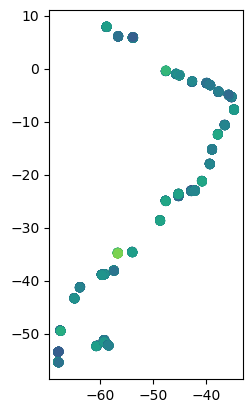
    history:                 [{'program': 'xcube_cci.chunkstore.CciChunkStore...

xarray.Dataset

• Dimensions:
  • nbpoints: 2066
  • nbmonth: 216
  • bnds: 2
• Coordinates: (3)
  • geometry
    (nbpoints)
    object
    POINT (-67.60308074951172 -49.39...

    array([<POINT (-67.603 -49.397)>, <POINT (-67.601 -49.4)>,
           <POINT (-67.598 -49.402)>, ..., <POINT (-34.747 -7.808)>,
           <POINT (-34.746 -7.81)>, <POINT (-34.745 -7.813)>], dtype=object)

  • nbmonth
    (nbmonth)
    datetime64[ns]
    2002-01-16T12:00:00 ... 2019-12-...

    standard_name :

    nbmonth

    bounds :

    nbmonth_bnds

    array(['2002-01-16T12:00:00.000000000', '2002-02-15T00:00:00.000000000',
           '2002-03-16T12:00:00.000000000', ..., '2019-10-16T12:00:00.000000000',
           '2019-11-16T00:00:00.000000000', '2019-12-16T12:00:00.000000000'],
          dtype='datetime64[ns]')

  • nbmonth_bnds
    (nbmonth, bnds)
    datetime64[ns]
    dask.array<chunksize=(216, 2), meta=np.ndarray>

    standard_name :

    nbmonth_bnds

    Array Chunk Bytes 3.38 kiB 3.38 kiB Shape (216, 2) (216, 2) Dask graph 1 chunks in 2 graph layers Data type datetime64[ns] numpy.ndarray

• Data variables: (6)
  • distance_to_coast
    (nbpoints)
    float32
    dask.array<chunksize=(50,), meta=np.ndarray>

    long_name :

    Distance to GSHHS 1.3 coastline

    units :

    m

    distance_to_coast_min :

    3299.2

    distance_to_coast_max :

    1.84467e+19

    comment :

    Distance along track to a reference point at the coast

    orig_data_type :

    float32

    fill_value :

    1.844674e+19

    size :

    2066

    shape :

    [2066]

    chunk_sizes :

    [50]

    file_chunk_sizes :

    [50]

    data_type :

    float32

    dimensions :

    ['nbpoints']

    file_dimensions :

    ['nbpoints']

    Array Chunk Bytes 8.07 kiB 200 B Shape (2066,) (50,) Dask graph 42 chunks in 2 graph layers Data type float32 numpy.ndarray

  • lat
    ()
    float64
    ...

    shape :

    []

    size :

    1

    chunk_sizes :

    []

    [1 values with dtype=float64]

  • local_sla_trend
    (nbpoints)
    float32
    dask.array<chunksize=(50,), meta=np.ndarray>

    long_name :

    Geographical distribution of sea level trends

    standard_name :

    tendency_of_sea_surface_height_above_sea_level

    units :

    mm/year

    comment :

    Sea level trends computed from X-TRACK/ALES monthly sea level anomalies between 2002-01-01 and 2019-12-31

    orig_data_type :

    float32

    fill_value :

    1.844674e+19

    size :

    2066

    shape :

    [2066]

    chunk_sizes :

    [50]

    file_chunk_sizes :

    [50]

    data_type :

    float32

    dimensions :

    ['nbpoints']

    file_dimensions :

    ['nbpoints']

    Array Chunk Bytes 8.07 kiB 200 B Shape (2066,) (50,) Dask graph 42 chunks in 2 graph layers Data type float32 numpy.ndarray

  • local_sla_trend_error
    (nbpoints)
    float32
    dask.array<chunksize=(50,), meta=np.ndarray>

    long_name :

    Geographical distribution of sea level trends errors

    units :

    mm/year

    orig_data_type :

    float32

    fill_value :

    1.844674e+19

    size :

    2066

    shape :

    [2066]

    chunk_sizes :

    [50]

    file_chunk_sizes :

    [50]

    data_type :

    float32

    dimensions :

    ['nbpoints']

    file_dimensions :

    ['nbpoints']

    Array Chunk Bytes 8.07 kiB 200 B Shape (2066,) (50,) Dask graph 42 chunks in 2 graph layers Data type float32 numpy.ndarray

  • lon
    ()
    float64
    ...

    shape :

    []

    size :

    1

    chunk_sizes :

    []

    [1 values with dtype=float64]

  • sla
    (nbpoints, nbmonth)
    float32
    dask.array<chunksize=(50, 216), meta=np.ndarray>

    units :

    m

    standard_name :

    sea_surface_height_above_mean_sea_level

    comment :

    The sla are monthly averaged and annual and semi-annual cycles are removed. sla = altitude of satellite - 20 Hz Ku band ALES corrected altimeter range (Passaro et al. 2014) - altimeter ionospheric correction on Ku band (From dual-frequency altimeter range measurements) - model dry tropospheric correction (From ECMWF model) - GPD+ wet tropospheric correction (Fernandes et al. 2016) - sea state bias correction in Ku band (ALES retracking, Passaro et al. 2014) - solid earth tide height (From RADS, tide potential model, Cartwright and Taylor 1971, Cartwright and Eden 1973) - geocentric ocean tide (FES 2014 from RADS, Carrere et al. 2012) - geocentric pole tide height (Wahr 1985) - Atmospheric correction (From RADS, Carrere and Lyard 2003) - X-TRACK mean sea surface (Birol et al. 2017). Each corrective term is edited following Birol et al. 2017.

    orig_data_type :

    float32

    fill_value :

    1.844674e+19

    size :

    446256

    shape :

    [2066, 216]

    chunk_sizes :

    [50, 216]

    file_chunk_sizes :

    [50, 216]

    data_type :

    float32

    dimensions :

    ['nbpoints', 'nbmonth']

    file_dimensions :

    ['nbpoints', 'nbmonth']

    Array Chunk Bytes 1.70 MiB 42.19 kiB Shape (2066, 216) (50, 216) Dask graph 42 chunks in 2 graph layers Data type float32 numpy.ndarray

• Indexes: (2)
  • nbmonth
    PandasIndex

    PandasIndex(DatetimeIndex(['2002-01-16 12:00:00', '2002-02-15 00:00:00',
                   '2002-03-16 12:00:00', '2002-04-16 00:00:00',
                   '2002-05-16 12:00:00', '2002-06-16 00:00:00',
                   '2002-07-16 12:00:00', '2002-08-16 12:00:00',
                   '2002-09-16 00:00:00', '2002-10-16 12:00:00',
                   ...
                   '2019-03-16 12:00:00', '2019-04-16 00:00:00',
                   '2019-05-16 12:00:00', '2019-06-16 00:00:00',
                   '2019-07-16 12:00:00', '2019-08-16 12:00:00',
                   '2019-09-16 00:00:00', '2019-10-16 12:00:00',
                   '2019-11-16 00:00:00', '2019-12-16 12:00:00'],
                  dtype='datetime64[ns]', name='nbmonth', length=216, freq=None))

  • geometry
    GeometryIndex (crs=None)

    GeometryIndex(
        [<POINT (-67.603 -49.397)>
         <POINT (-67.601 -49.4)>
         <POINT (-67.598 -49.402)>
         <POINT (-67.596 -49.404)>
         ...
         <POINT (-34.748 -7.805)>
         <POINT (-34.747 -7.808)>
         <POINT (-34.746 -7.81)>
         <POINT (-34.745 -7.813)>],
        crs=None)

• Attributes: (8)

  Conventions :

  CF-1.7

  title :

  esacci.SEALEVEL.mon.IND.MSLTR.multi-sensor.multi-platform.MERGED.2-2.ASA

  date_created :

  2025-12-04T11:41:39.087709

  processing_level :

  IND

  time_coverage_start :

  2002-01-01T00:00:00

  time_coverage_end :

  2020-01-01T00:00:00

  time_coverage_duration :

  P6574DT0H0M0S

  history :

  [{'program': 'xcube_cci.chunkstore.CciChunkStore', 'cube_params': {'time_range': ['2002-01-01T00:00:00', '2019-12-31T23:59:59'], 'variable_names': ['distance_to_coast', 'lat', 'lon', 'local_sla_trend', 'local_sla_trend_error', 'sla']}}]

We see that the resulting dataset has a geometry coordinate which consists of single points. We may plot a variable which only has a single geometric dimension like this:

import geopandas as gpd
gdf = gpd.GeoDataFrame(sl_ds[["geometry", "local_sla_trend"]].to_dataframe())
gdf.plot(column="local_sla_trend")

<Axes: >

We may also plot variables which have values along the temporal dimension. We can do so like this:

gdf2 = gpd.GeoDataFrame(sl_ds[["geometry", "sla", "nbmonth"]].to_dataframe())
gdf2.xs("2019-09-16 00:00:00", level="nbmonth").plot(column="sla")

<Axes: >

sl_ds = cci_store.open_data(
    "esacci.SEALEVEL.mon.IND.MSLTR.multi-sensor.multi-platform.MERGED.2-2.ASA"
)
gdf = gpd.GeoDataFrame(sl_ds[["geometry", "local_sla_trend"]].to_dataframe())
gdf.plot(column="local_sla_trend")

<Axes: >