4.2.1.11. ESA CCI Toolbox Data Tree Access
Some of the data from the Open Data Portal is provided through the Toolbox in the form of DataTrees. DataTrees are basically a collection of datasets, where each dataset may be accessed through an identifier. This structure is applied to all gridded data that is subdivided into regions. As each of these region-specific datasets is a standard dataset, all toolbox operations can be applied to them.
This notebook shall serve to show what CCI datasets are concerned and how they can be opened.
To run this Notebook, make sure the ESA CCI Toolbox is setup correctly.
We start, as usual, by opening the standard esa-cci data store.
[1]:
from xcube.core.store import new_data_store

cci_store = new_data_store('esa-cci')
We list the available data types of the store to make sure ‘datatree’ is included in the list.
[2]:
cci_store.get_data_types()
[2]:
('dataset', 'geodataframe', 'vectordatacube', 'datatree')
As datatrees are provided, we can ask which datasets are actually provided in this form.
[3]:
list(cci_store.get_data_ids(data_type="datatree"))
[3]:
['esacci.FIRE.mon.L3S.BA.MODIS.Terra.MODIS_TERRA.v5-1.pixel',
 'esacci.FIRE.mon.L3S.BA.multi-sensor.multi-platform.SYN.v1-1.pixel',
 'esacci.FIRE.mon.L3S.BA.MSI-(Sentinel-2).Sentinel-2A.MSI.2-0.pixel',
 'esacci.FIRE.mon.L3S.BA.MSI-(Sentinel-2).Sentinel-2A.MSI.v1-1.pixel',
 'esacci.LC.yr.L4.Map.multi-sensor.multi-platform.HRLC10-A03.v1-2.Siberia',
 'esacci.LC.yr.L4.Map.multi-sensor.multi-platform.HRLC10-A02.v1-2.Amazonia',
 'esacci.LC.yr.L4.Map.multi-sensor.multi-platform.HRLC10-A01.v1-2.Africa',
 'esacci.LC.5-yrs.L4.Map.multi-sensor.multi-platform.HRLC30-A03.v1-2.Siberia',
 'esacci.LC.5-yrs.L4.Map.multi-sensor.multi-platform.HRLC30-A02.v1-2.Amazonia',
 'esacci.LC.5-yrs.L4.Map.multi-sensor.multi-platform.HRLC30-A01.v1-2.Africa',
 'esacci.LC.5-yrs.L4.CHANGE.multi-sensor.multi-platform.HRLCC30-A03.v1-2.Siberia',
 'esacci.LC.5-yrs.L4.CHANGE.multi-sensor.multi-platform.HRLCC30-A02.v1-2.Amazonia',
 'esacci.LC.5-yrs.L4.CHANGE.multi-sensor.multi-platform.HRLCC30-A01.v1-2.Africa',
 'esacci.VEGETATION.5-days.L3S.VP_PRODUCTS.VEGETATION.SPOT-5.MERGED.v1-0.r1',
 'esacci.VEGETATION.5-days.L3S.VP_PRODUCTS.VEGETATION.multi-platform.MERGED.v1-0.r1',
 'esacci.VEGETATION.5-days.L3S.VP_PRODUCTS.Végétation-P.PROBA-V.MERGED.v1-0.r1',
 'esacci.VEGETATION.5-days.L3S.VP_PRODUCTS.multi-sensor.multi-platform.MERGED.v1-0.r1']
So, datatrees are provided for three ECVs: FIRE, LC, and VEGETATION. To fully show the use of datatrees, we will open FIRE and VEGETATION data.
4.2.1.11.1. Opening FIRE Data
We start with opening one of the FIRE datasets.
[4]:
fire_dataset = "esacci.FIRE.mon.L3S.BA.MODIS.Terra.MODIS_TERRA.v5-1.pixel"
As first step, we have a look at the potential opener parameters.
[5]:
cci_store.get_open_data_params_schema(fire_dataset)
[5]:
<xcube.util.jsonschema.JsonObjectSchema at 0x78c9da7f2a50>
One entry that we don’t see when opening datasets of other type is the property place_names. If we extend this, we see a listing of Areas 1 to 6. Each of these identifiers stands for a different area. We can either open the data tree with all areas or pass a subset of this list as a parameter to only retrieve the area we are interested in. This will also increase performance.
[6]:
places = ["AREA_1"]
[7]:
fire_dt = cci_store.open_data(
    fire_dataset,
    place_names=places
)
fire_dt
[7]:
<xarray.DataTree 'esacci.FIRE.mon.L3S.BA.MODIS.Terra.MODIS_TERRA.v5-1.pixel'>
Group: /
└── Group: /
        Dimensions:    (time: 264, y: 28499, x: 57888, bnds: 2)
        Coordinates:
          * time       (time) datetime64[ns] 2kB 2001-01-16T12:00:00 ... 2022-12-16T1...
            time_bnds  (time, bnds) datetime64[ns] 4kB dask.array<chunksize=(264, 2), meta=np.ndarray>
          * x          (x) float64 463kB -180.0 -180.0 -180.0 ... -50.0 -50.0 -50.0
          * y          (y) float64 228kB 83.0 83.0 82.99 82.99 ... 19.01 19.0 19.0 19.0
        Dimensions without coordinates: bnds
        Data variables:
            CL         (time, y, x) uint8 436GB dask.array<chunksize=(1, 28499, 144), meta=np.ndarray>
            JD         (time, y, x) int16 871GB dask.array<chunksize=(1, 28499, 144), meta=np.ndarray>
            LC         (time, y, x) uint8 436GB dask.array<chunksize=(1, 28499, 144), meta=np.ndarray>
        Attributes:
            Conventions:             CF-1.7
            title:                   esacci.FIRE.mon.L3S.BA.MODIS.Terra.MODIS_TERRA.v...
            date_created:            2025-12-08T12:04:28.461120
            processing_level:        L3S
            time_coverage_start:     2001-01-01T00:00:00
            time_coverage_end:       2023-01-01T00:00:00
            time_coverage_duration:  P8035DT0H0M0S
            history:                 [{'program': 'xcube_cci.chunkstore.CciChunkStore...
We can see which datasets are available by asking for its keys.
[8]:
list(fire_dt.keys())
[8]:
['AREA_1']
As expected, it is the place(s) we had requested. We can now retrieve a dataset from any of the keys.
[9]:
ds = fire_dt.get(places[0]).to_dataset()
ds
[9]:
<xarray.Dataset> Size: 2TB
Dimensions:    (time: 264, y: 28499, x: 57888, bnds: 2)
Coordinates:
  * time       (time) datetime64[ns] 2kB 2001-01-16T12:00:00 ... 2022-12-16T1...
    time_bnds  (time, bnds) datetime64[ns] 4kB dask.array<chunksize=(264, 2), meta=np.ndarray>
  * x          (x) float64 463kB -180.0 -180.0 -180.0 ... -50.0 -50.0 -50.0
  * y          (y) float64 228kB 83.0 83.0 82.99 82.99 ... 19.01 19.0 19.0 19.0
Dimensions without coordinates: bnds
Data variables:
    CL         (time, y, x) uint8 436GB dask.array<chunksize=(1, 28499, 144), meta=np.ndarray>
    JD         (time, y, x) int16 871GB dask.array<chunksize=(1, 28499, 144), meta=np.ndarray>
    LC         (time, y, x) uint8 436GB dask.array<chunksize=(1, 28499, 144), meta=np.ndarray>
Attributes:
    Conventions:             CF-1.7
    title:                   esacci.FIRE.mon.L3S.BA.MODIS.Terra.MODIS_TERRA.v...
    date_created:            2025-12-08T12:04:28.461120
    processing_level:        L3S
    time_coverage_start:     2001-01-01T00:00:00
    time_coverage_end:       2023-01-01T00:00:00
    time_coverage_duration:  P8035DT0H0M0S
history: [{'program': 'xcube_cci.chunkstore.CciChunkStore...- time: 264
- y: 28499
- x: 57888
- bnds: 2
- time(time)datetime64[ns]2001-01-16T12:00:00 ... 2022-12-...
- standard_name :
- time
- bounds :
- time_bnds
array(['2001-01-16T12:00:00.000000000', '2001-02-15T00:00:00.000000000', '2001-03-16T12:00:00.000000000', ..., '2022-10-16T12:00:00.000000000', '2022-11-16T00:00:00.000000000', '2022-12-16T12:00:00.000000000'], dtype='datetime64[ns]') - time_bnds(time, bnds)datetime64[ns]dask.array<chunksize=(264, 2), meta=np.ndarray>
- standard_name :
- time_bnds
Array Chunk Bytes 4.12 kiB 4.12 kiB Shape (264, 2) (264, 2) Dask graph 1 chunks in 2 graph layers Data type datetime64[ns] numpy.ndarray - x(x)float64-180.0 -180.0 ... -50.0 -50.0
- dimensions :
- x
- file_dimensions :
- x
- size :
- 57888
- shape :
- [57888]
- data_type :
- float64
- chunk_sizes :
- [57888]
- file_chunk_sizes :
- [57888]
array([-179.998877, -179.996631, -179.994386, ..., -50.004616, -50.00237 , -50.000125]) - y(y)float6483.0 83.0 82.99 ... 19.0 19.0 19.0
- dimensions :
- y
- file_dimensions :
- y
- size :
- 28499
- shape :
- [28499]
- data_type :
- float64
- chunk_sizes :
- [28499]
- file_chunk_sizes :
- [28499]
array([82.998927, 82.996681, 82.994436, ..., 19.004516, 19.002271, 19.000025])
- CL(time, y, x)uint8dask.array<chunksize=(1, 28499, 144), meta=np.ndarray>
- dimensions :
- ['time', 'y', 'x']
- file_dimensions :
- ['time', 'y', 'x']
- size :
- 435534029568
- shape :
- [264, 28499, 57888]
- data_type :
- uint8
- chunk_sizes :
- [1, 28499, 144]
- file_chunk_sizes :
- [1, 28499, 144]
Array Chunk Bytes 405.62 GiB 3.91 MiB Shape (264, 28499, 57888) (1, 28499, 144) Dask graph 106128 chunks in 2 graph layers Data type uint8 numpy.ndarray - JD(time, y, x)int16dask.array<chunksize=(1, 28499, 144), meta=np.ndarray>
- dimensions :
- ['time', 'y', 'x']
- file_dimensions :
- ['time', 'y', 'x']
- size :
- 435534029568
- shape :
- [264, 28499, 57888]
- data_type :
- int16
- chunk_sizes :
- [1, 28499, 144]
- file_chunk_sizes :
- [1, 28499, 144]
Array Chunk Bytes 811.25 GiB 7.83 MiB Shape (264, 28499, 57888) (1, 28499, 144) Dask graph 106128 chunks in 2 graph layers Data type int16 numpy.ndarray - LC(time, y, x)uint8dask.array<chunksize=(1, 28499, 144), meta=np.ndarray>
- dimensions :
- ['time', 'y', 'x']
- file_dimensions :
- ['time', 'y', 'x']
- size :
- 435534029568
- shape :
- [264, 28499, 57888]
- data_type :
- uint8
- chunk_sizes :
- [1, 28499, 144]
- file_chunk_sizes :
- [1, 28499, 144]
Array Chunk Bytes 405.62 GiB 3.91 MiB Shape (264, 28499, 57888) (1, 28499, 144) Dask graph 106128 chunks in 2 graph layers Data type uint8 numpy.ndarray
- timePandasIndex
PandasIndex(DatetimeIndex(['2001-01-16 12:00:00', '2001-02-15 00:00:00', '2001-03-16 12:00:00', '2001-04-16 00:00:00', '2001-05-16 12:00:00', '2001-06-16 00:00:00', '2001-07-16 12:00:00', '2001-08-16 12:00:00', '2001-09-16 00:00:00', '2001-10-16 12:00:00', ... '2022-03-16 12:00:00', '2022-04-16 00:00:00', '2022-05-16 12:00:00', '2022-06-16 00:00:00', '2022-07-16 12:00:00', '2022-08-16 12:00:00', '2022-09-16 00:00:00', '2022-10-16 12:00:00', '2022-11-16 00:00:00', '2022-12-16 12:00:00'], dtype='datetime64[ns]', name='time', length=264, freq=None)) - xPandasIndex
PandasIndex(Index([-179.99887713344646, -179.99663140033937, -179.99438566723228, -179.9921399341252, -179.9898942010181, -179.98764846791101, -179.98540273480393, -179.98315700169684, -179.98091126858975, -179.97866553548266, ... -50.020336361395664, -50.018090628288576, -50.01584489518149, -50.0135991620744, -50.01135342896731, -50.00910769586022, -50.006861962753135, -50.00461622964605, -50.00237049653896, -50.00012476343187], dtype='float64', name='x', length=57888)) - yPandasIndex
PandasIndex(Index([ 82.99892703862662,  82.99668130551952,  82.99443557241243,
        82.99218983930533,  82.98994410619824,  82.98769837309113,
        82.98545263998403,  82.98320690687694,  82.98096117376984,
        82.97871544066275,
       ...
       19.020236550553953, 19.017990817446858, 19.015745084339763,
        19.01349935123266, 19.011253618125565,  19.00900788501847,
       19.006762151911374,  19.00451641880428, 19.002270685697184,
        19.00002495259008],
      dtype='float64', name='y', length=28499))
- Conventions :
- CF-1.7
- title :
- esacci.FIRE.mon.L3S.BA.MODIS.Terra.MODIS_TERRA.v5-1.pixel~AREA_1
- date_created :
- 2025-12-08T12:04:28.461120
- processing_level :
- L3S
- time_coverage_start :
- 2001-01-01T00:00:00
- time_coverage_end :
- 2023-01-01T00:00:00
- time_coverage_duration :
- P8035DT0H0M0S
- history :
- [{'program': 'xcube_cci.chunkstore.CciChunkStore', 'cube_params': {'time_range': ['2001-01-01T00:00:00', '2022-12-31T23:59:59'], 'variable_names': ['JD', 'CL', 'LC']}}]
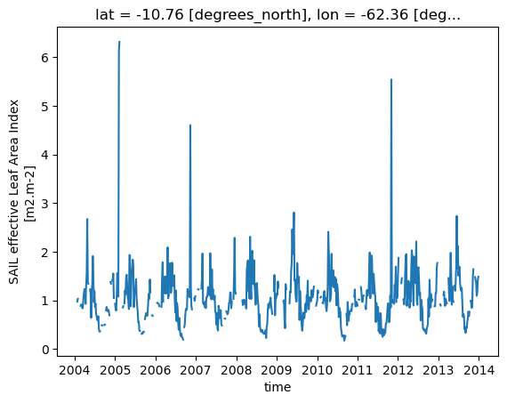
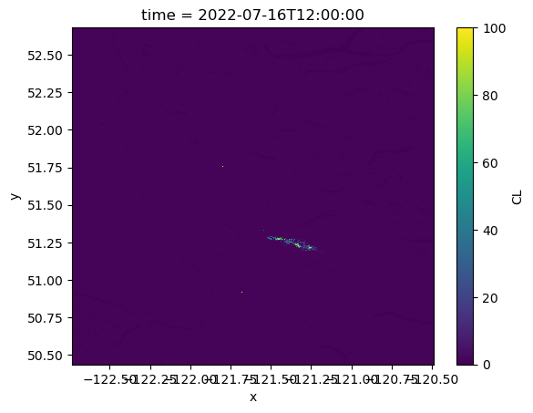
And, of course, we can open and plot any of the data variables:
[10]:
ds.CL.isel({"time": -6, "x": slice(25500, 26500), "y": slice(13500, 14500)}).plot()
[10]:
<matplotlib.collections.QuadMesh at 0x78c9be0ebcb0>
4.2.1.11.2. Opening VEGETATION Data
We continue by opening a VEGETATION data set. What’s particular about this dataset is that it offers a lot of different sites, as becomes apparent from looking at the places in the schema properties
[11]:
vegetation_ds = "esacci.VEGETATION.5-days.L3S.VP_PRODUCTS.VEGETATION.SPOT-5.MERGED.v1-0.r1"
[12]:
cci_store.get_open_data_params_schema(vegetation_ds)
[12]:
<xcube.util.jsonschema.JsonObjectSchema at 0x78c9e3776a50>
We can pick any of those sites and use them to open the data tree.
[13]:
places = ["site_00001_ABRACOS_HILL", "site_00021_BASKIN"]
[14]:
abracos = cci_store.open_data(
    vegetation_ds,
    place_names=places
)
abracos
[14]:
<xarray.DataTree 'esacci.VEGETATION.5-days.L3S.VP_PRODUCTS.VEGETATION.SPOT-5.MERGED.v1-0.r1'>
Group: /
├── Group: /
│       Dimensions:                   (time: 730, lat: 3, lon: 3, nbnds: 2, bnds: 2)
│       Coordinates:
│         * lat                       (lat) float32 12B -10.75 -10.76 -10.77
│           lat_bnds                  (lat, nbnds) float32 24B dask.array<chunksize=(3, 2), meta=np.ndarray>
│         * lon                       (lon) float32 12B -62.37 -62.36 -62.35
│           lon_bnds                  (lon, nbnds) float32 24B dask.array<chunksize=(3, 2), meta=np.ndarray>
│         * time                      (time) datetime64[ns] 6kB 2004-01-01T11:59:59 ....
│           time_bnds                 (time, bnds) datetime64[ns] 12kB dask.array<chunksize=(730, 2), meta=np.ndarray>
│       Dimensions without coordinates: nbnds, bnds
│       Data variables: (12/69)
│           BHR_NIR                   (time, lat, lon) float64 53kB dask.array<chunksize=(73, 3, 3), meta=np.ndarray>
│           BHR_NIR_BHR_SW_correl     (time, lat, lon) float64 53kB dask.array<chunksize=(73, 3, 3), meta=np.ndarray>
│           BHR_NIR_DHR_NIR_correl    (time, lat, lon) float64 53kB dask.array<chunksize=(73, 3, 3), meta=np.ndarray>
│           BHR_NIR_DHR_SW_correl     (time, lat, lon) float64 53kB dask.array<chunksize=(73, 3, 3), meta=np.ndarray>
│           BHR_NIR_DHR_VIS_correl    (time, lat, lon) float64 53kB dask.array<chunksize=(73, 3, 3), meta=np.ndarray>
│           BHR_NIR_ERR               (time, lat, lon) float64 53kB dask.array<chunksize=(73, 3, 3), meta=np.ndarray>
│           ...                        ...
│           fAPAR_DHR_VIS_correl      (time, lat, lon) float64 53kB dask.array<chunksize=(73, 3, 3), meta=np.ndarray>
│           fAPAR_ERR                 (time, lat, lon) float64 53kB dask.array<chunksize=(73, 3, 3), meta=np.ndarray>
│           fAPAR_fAPAR_Cab_correl    (time, lat, lon) float64 53kB dask.array<chunksize=(73, 3, 3), meta=np.ndarray>
│           invcode                   (time, lat, lon) float64 53kB dask.array<chunksize=(73, 3, 3), meta=np.ndarray>
│           n_bands_used              (time, lat, lon) float64 53kB dask.array<chunksize=(73, 3, 3), meta=np.ndarray>
│           p_chisquare               (time, lat, lon) float64 53kB dask.array<chunksize=(73, 3, 3), meta=np.ndarray>
│       Attributes:
│           Conventions:             CF-1.7
│           title:                   esacci.VEGETATION.5-days.L3S.VP_PRODUCTS.VEGETAT...
│           date_created:            2025-12-08T12:10:15.529611
│           processing_level:        L3S
│           time_coverage_start:     2004-01-01T00:00:00
│           time_coverage_end:       2013-12-27T23:59:59
│           time_coverage_duration:  P3648DT23H59M59S
│           history:                 [{'program': 'xcube_cci.chunkstore.CciChunkStore...
└── Group: /
        Dimensions:                   (time: 730, lat: 3, lon: 3, nbnds: 2, bnds: 2)
        Coordinates:
          * lat                       (lat) float32 12B 32.29 32.29 32.28
            lat_bnds                  (lat, nbnds) float32 24B dask.array<chunksize=(3, 2), meta=np.ndarray>
          * lon                       (lon) float32 12B -91.75 -91.74 -91.73
            lon_bnds                  (lon, nbnds) float32 24B dask.array<chunksize=(3, 2), meta=np.ndarray>
          * time                      (time) datetime64[ns] 6kB 2004-01-01T11:59:59 ....
            time_bnds                 (time, bnds) datetime64[ns] 12kB dask.array<chunksize=(730, 2), meta=np.ndarray>
        Dimensions without coordinates: nbnds, bnds
        Data variables: (12/69)
            BHR_NIR                   (time, lat, lon) float64 53kB dask.array<chunksize=(73, 3, 3), meta=np.ndarray>
            BHR_NIR_BHR_SW_correl     (time, lat, lon) float64 53kB dask.array<chunksize=(73, 3, 3), meta=np.ndarray>
            BHR_NIR_DHR_NIR_correl    (time, lat, lon) float64 53kB dask.array<chunksize=(73, 3, 3), meta=np.ndarray>
            BHR_NIR_DHR_SW_correl     (time, lat, lon) float64 53kB dask.array<chunksize=(73, 3, 3), meta=np.ndarray>
            BHR_NIR_DHR_VIS_correl    (time, lat, lon) float64 53kB dask.array<chunksize=(73, 3, 3), meta=np.ndarray>
            BHR_NIR_ERR               (time, lat, lon) float64 53kB dask.array<chunksize=(73, 3, 3), meta=np.ndarray>
            ...                        ...
            fAPAR_DHR_VIS_correl      (time, lat, lon) float64 53kB dask.array<chunksize=(73, 3, 3), meta=np.ndarray>
            fAPAR_ERR                 (time, lat, lon) float64 53kB dask.array<chunksize=(73, 3, 3), meta=np.ndarray>
            fAPAR_fAPAR_Cab_correl    (time, lat, lon) float64 53kB dask.array<chunksize=(73, 3, 3), meta=np.ndarray>
            invcode                   (time, lat, lon) float64 53kB dask.array<chunksize=(73, 3, 3), meta=np.ndarray>
            n_bands_used              (time, lat, lon) float64 53kB dask.array<chunksize=(73, 3, 3), meta=np.ndarray>
            p_chisquare               (time, lat, lon) float64 53kB dask.array<chunksize=(73, 3, 3), meta=np.ndarray>
        Attributes:
            Conventions:             CF-1.7
            title:                   esacci.VEGETATION.5-days.L3S.VP_PRODUCTS.VEGETAT...
            date_created:            2025-12-08T12:10:36.067594
            processing_level:        L3S
            time_coverage_start:     2004-01-01T00:00:00
            time_coverage_end:       2013-12-27T23:59:59
            time_coverage_duration:  P3648DT23H59M59S
            history:                 [{'program': 'xcube_cci.chunkstore.CciChunkStore...
Again, we see check that the correct places are provided.
[15]:
list(abracos.keys())
[15]:
['site_00001_ABRACOS_HILL', 'site_00021_BASKIN']
We now open one of these datasets.
[16]:
ds = abracos.get(places[0]).to_dataset()
ds
[16]:
<xarray.Dataset> Size: 4MB
Dimensions:                   (time: 730, lat: 3, lon: 3, nbnds: 2, bnds: 2)
Coordinates:
  * lat                       (lat) float32 12B -10.75 -10.76 -10.77
    lat_bnds                  (lat, nbnds) float32 24B dask.array<chunksize=(3, 2), meta=np.ndarray>
  * lon                       (lon) float32 12B -62.37 -62.36 -62.35
    lon_bnds                  (lon, nbnds) float32 24B dask.array<chunksize=(3, 2), meta=np.ndarray>
  * time                      (time) datetime64[ns] 6kB 2004-01-01T11:59:59 ....
    time_bnds                 (time, bnds) datetime64[ns] 12kB dask.array<chunksize=(730, 2), meta=np.ndarray>
Dimensions without coordinates: nbnds, bnds
Data variables: (12/69)
    BHR_NIR                   (time, lat, lon) float64 53kB dask.array<chunksize=(73, 3, 3), meta=np.ndarray>
    BHR_NIR_BHR_SW_correl     (time, lat, lon) float64 53kB dask.array<chunksize=(73, 3, 3), meta=np.ndarray>
    BHR_NIR_DHR_NIR_correl    (time, lat, lon) float64 53kB dask.array<chunksize=(73, 3, 3), meta=np.ndarray>
    BHR_NIR_DHR_SW_correl     (time, lat, lon) float64 53kB dask.array<chunksize=(73, 3, 3), meta=np.ndarray>
    BHR_NIR_DHR_VIS_correl    (time, lat, lon) float64 53kB dask.array<chunksize=(73, 3, 3), meta=np.ndarray>
    BHR_NIR_ERR               (time, lat, lon) float64 53kB dask.array<chunksize=(73, 3, 3), meta=np.ndarray>
    ...                        ...
    fAPAR_DHR_VIS_correl      (time, lat, lon) float64 53kB dask.array<chunksize=(73, 3, 3), meta=np.ndarray>
    fAPAR_ERR                 (time, lat, lon) float64 53kB dask.array<chunksize=(73, 3, 3), meta=np.ndarray>
    fAPAR_fAPAR_Cab_correl    (time, lat, lon) float64 53kB dask.array<chunksize=(73, 3, 3), meta=np.ndarray>
    invcode                   (time, lat, lon) float64 53kB dask.array<chunksize=(73, 3, 3), meta=np.ndarray>
    n_bands_used              (time, lat, lon) float64 53kB dask.array<chunksize=(73, 3, 3), meta=np.ndarray>
    p_chisquare               (time, lat, lon) float64 53kB dask.array<chunksize=(73, 3, 3), meta=np.ndarray>
Attributes:
    Conventions:             CF-1.7
    title:                   esacci.VEGETATION.5-days.L3S.VP_PRODUCTS.VEGETAT...
    date_created:            2025-12-08T12:10:15.529611
    processing_level:        L3S
    time_coverage_start:     2004-01-01T00:00:00
    time_coverage_end:       2013-12-27T23:59:59
    time_coverage_duration:  P3648DT23H59M59S
history: [{'program': 'xcube_cci.chunkstore.CciChunkStore...- time: 730
- lat: 3
- lon: 3
- nbnds: 2
- bnds: 2
- lat(lat)float32-10.75 -10.76 -10.77
- standard_name :
- latitude
- long_name :
- latitude
- units :
- degrees_north
- axis :
- Y
- bounds :
- lat_bnds
- orig_data_type :
- float32
- fill_value :
- nan
- size :
- 3
- shape :
- [3]
- chunk_sizes :
- [3]
- file_chunk_sizes :
- [3]
- data_type :
- float32
- dimensions :
- ['lat']
- file_dimensions :
- ['lat']
array([-10.75 , -10.758928, -10.767858], dtype=float32)
- lat_bnds(lat, nbnds)float32dask.array<chunksize=(3, 2), meta=np.ndarray>
- orig_data_type :
- float32
- fill_value :
- nan
- size :
- 6
- shape :
- [3, 2]
- chunk_sizes :
- [3, 2]
- file_chunk_sizes :
- [3, 2]
- data_type :
- float32
- dimensions :
- ['lat', 'nbnds']
- file_dimensions :
- ['lat', 'nbnds']
Array Chunk Bytes 24 B 24 B Shape (3, 2) (3, 2) Dask graph 1 chunks in 2 graph layers Data type float32 numpy.ndarray - lon(lon)float32-62.37 -62.36 -62.35
- standard_name :
- longitude
- long_name :
- longitude
- units :
- degrees_east
- axis :
- X
- bounds :
- lon_bnds
- orig_data_type :
- float32
- fill_value :
- nan
- size :
- 3
- shape :
- [3]
- chunk_sizes :
- [3]
- file_chunk_sizes :
- [3]
- data_type :
- float32
- dimensions :
- ['lon']
- file_dimensions :
- ['lon']
array([-62.36607 , -62.357143, -62.348213], dtype=float32)
- lon_bnds(lon, nbnds)float32dask.array<chunksize=(3, 2), meta=np.ndarray>
- orig_data_type :
- float32
- fill_value :
- nan
- size :
- 6
- shape :
- [3, 2]
- chunk_sizes :
- [3, 2]
- file_chunk_sizes :
- [3, 2]
- data_type :
- float32
- dimensions :
- ['lon', 'nbnds']
- file_dimensions :
- ['lon', 'nbnds']
Array Chunk Bytes 24 B 24 B Shape (3, 2) (3, 2) Dask graph 1 chunks in 2 graph layers Data type float32 numpy.ndarray - time(time)datetime64[ns]2004-01-01T11:59:59 ... 2013-12-...
- standard_name :
- time
- bounds :
- time_bnds
array(['2004-01-01T11:59:59.000000000', '2004-01-06T11:59:59.000000000', '2004-01-11T11:59:59.000000000', ..., '2013-12-17T11:59:59.000000000', '2013-12-22T11:59:59.000000000', '2013-12-27T11:59:59.000000000'], dtype='datetime64[ns]') - time_bnds(time, bnds)datetime64[ns]dask.array<chunksize=(730, 2), meta=np.ndarray>
- standard_name :
- time_bnds
Array Chunk Bytes 11.41 kiB 11.41 kiB Shape (730, 2) (730, 2) Dask graph 1 chunks in 2 graph layers Data type datetime64[ns] numpy.ndarray
- BHR_NIR(time, lat, lon)float64dask.array<chunksize=(73, 3, 3), meta=np.ndarray>
- long_name :
- bi-hemispherical reflectance (albedo) in the near infra-red range
- units :
- 1
- ancillary_variables :
- BHR_NIR_ERR invcode p_chisquare LAI_BHR_NIR_correl fAPAR_BHR_NIR_correl fAPAR_Cab_BHR_NIR_correl Cab_BHR_NIR_correl BHR_VIS_BHR_NIR_correl BHR_NIR_BHR_SW_correl BHR_NIR_DHR_VIS_correl BHR_NIR_DHR_NIR_correl BHR_NIR_DHR_SW_correl
- ancillary_roles :
- uncertainty, quality of the retrieval, quality of model fit, standard error correlation with LAI, standard error correlation with fAPAR, standard error correlation with fAPAR_Cab, standard error correlation with Cab, standard error correlation with BHR_VIS, standard error correlation with BHR_SW, standard error correlation with DHR_VIS, standard error correlation with DHR_NIR, standard error correlation with DHR_SW
- grid_mapping :
- crs
- valid_min :
- -32767
- valid_max :
- 32767
- orig_data_type :
- int16
- fill_value :
- -32768
- size :
- 6570
- shape :
- [730, 3, 3]
- chunk_sizes :
- [73, 3, 3]
- file_chunk_sizes :
- [73, 3, 3]
- data_type :
- int16
- dimensions :
- ['time', 'lat', 'lon']
- file_dimensions :
- ['time', 'lat', 'lon']
Array Chunk Bytes 51.33 kiB 5.13 kiB Shape (730, 3, 3) (73, 3, 3) Dask graph 10 chunks in 2 graph layers Data type float64 numpy.ndarray - BHR_NIR_BHR_SW_correl(time, lat, lon)float64dask.array<chunksize=(73, 3, 3), meta=np.ndarray>
- long_name :
- BHR_NIR BHR_SW standard_error_correlation
- units :
- 1
- grid_mapping :
- crs
- valid_min :
- -127
- valid_max :
- 127
- orig_data_type :
- uint8
- fill_value :
- 128
- size :
- 6570
- shape :
- [730, 3, 3]
- chunk_sizes :
- [73, 3, 3]
- file_chunk_sizes :
- [73, 3, 3]
- data_type :
- uint8
- dimensions :
- ['time', 'lat', 'lon']
- file_dimensions :
- ['time', 'lat', 'lon']
Array Chunk Bytes 51.33 kiB 5.13 kiB Shape (730, 3, 3) (73, 3, 3) Dask graph 10 chunks in 2 graph layers Data type float64 numpy.ndarray - BHR_NIR_DHR_NIR_correl(time, lat, lon)float64dask.array<chunksize=(73, 3, 3), meta=np.ndarray>
- long_name :
- BHR_NIR DHR_NIR standard_error_correlation
- units :
- 1
- grid_mapping :
- crs
- valid_min :
- -127
- valid_max :
- 127
- orig_data_type :
- uint8
- fill_value :
- 128
- size :
- 6570
- shape :
- [730, 3, 3]
- chunk_sizes :
- [73, 3, 3]
- file_chunk_sizes :
- [73, 3, 3]
- data_type :
- uint8
- dimensions :
- ['time', 'lat', 'lon']
- file_dimensions :
- ['time', 'lat', 'lon']
Array Chunk Bytes 51.33 kiB 5.13 kiB Shape (730, 3, 3) (73, 3, 3) Dask graph 10 chunks in 2 graph layers Data type float64 numpy.ndarray - BHR_NIR_DHR_SW_correl(time, lat, lon)float64dask.array<chunksize=(73, 3, 3), meta=np.ndarray>
- long_name :
- BHR_NIR DHR_SW standard_error_correlation
- units :
- 1
- grid_mapping :
- crs
- valid_min :
- -127
- valid_max :
- 127
- orig_data_type :
- uint8
- fill_value :
- 128
- size :
- 6570
- shape :
- [730, 3, 3]
- chunk_sizes :
- [73, 3, 3]
- file_chunk_sizes :
- [73, 3, 3]
- data_type :
- uint8
- dimensions :
- ['time', 'lat', 'lon']
- file_dimensions :
- ['time', 'lat', 'lon']
Array Chunk Bytes 51.33 kiB 5.13 kiB Shape (730, 3, 3) (73, 3, 3) Dask graph 10 chunks in 2 graph layers Data type float64 numpy.ndarray - BHR_NIR_DHR_VIS_correl(time, lat, lon)float64dask.array<chunksize=(73, 3, 3), meta=np.ndarray>
- long_name :
- BHR_NIR DHR_VIS standard_error_correlation
- units :
- 1
- grid_mapping :
- crs
- valid_min :
- -127
- valid_max :
- 127
- orig_data_type :
- uint8
- fill_value :
- 128
- size :
- 6570
- shape :
- [730, 3, 3]
- chunk_sizes :
- [73, 3, 3]
- file_chunk_sizes :
- [73, 3, 3]
- data_type :
- uint8
- dimensions :
- ['time', 'lat', 'lon']
- file_dimensions :
- ['time', 'lat', 'lon']
Array Chunk Bytes 51.33 kiB 5.13 kiB Shape (730, 3, 3) (73, 3, 3) Dask graph 10 chunks in 2 graph layers Data type float64 numpy.ndarray - BHR_NIR_ERR(time, lat, lon)float64dask.array<chunksize=(73, 3, 3), meta=np.ndarray>
- long_name :
- BHR_NIR standard_error
- units :
- 1
- grid_mapping :
- crs
- valid_min :
- -32767
- valid_max :
- 32767
- orig_data_type :
- int16
- fill_value :
- -32768
- size :
- 6570
- shape :
- [730, 3, 3]
- chunk_sizes :
- [73, 3, 3]
- file_chunk_sizes :
- [73, 3, 3]
- data_type :
- int16
- dimensions :
- ['time', 'lat', 'lon']
- file_dimensions :
- ['time', 'lat', 'lon']
Array Chunk Bytes 51.33 kiB 5.13 kiB Shape (730, 3, 3) (73, 3, 3) Dask graph 10 chunks in 2 graph layers Data type float64 numpy.ndarray - BHR_SW(time, lat, lon)float64dask.array<chunksize=(73, 3, 3), meta=np.ndarray>
- long_name :
- bi-hemispherical reflectance (albedo) in the shortwave range
- units :
- 1
- ancillary_variables :
- BHR_SW_ERR invcode p_chisquare LAI_BHR_SW_correl fAPAR_BHR_SW_correl fAPAR_Cab_BHR_SW_correl Cab_BHR_SW_correl BHR_VIS_BHR_SW_correl BHR_NIR_BHR_SW_correl BHR_SW_DHR_VIS_correl BHR_SW_DHR_NIR_correl BHR_SW_DHR_SW_correl
- ancillary_roles :
- uncertainty, quality of the retrieval, quality of model fit, standard error correlation with LAI, standard error correlation with fAPAR, standard error correlation with fAPAR_Cab, standard error correlation with Cab, standard error correlation with BHR_VIS, standard error correlation with BHR_NIR, standard error correlation with DHR_VIS, standard error correlation with DHR_NIR, standard error correlation with DHR_SW
- grid_mapping :
- crs
- valid_min :
- -32767
- valid_max :
- 32767
- orig_data_type :
- int16
- fill_value :
- -32768
- size :
- 6570
- shape :
- [730, 3, 3]
- chunk_sizes :
- [73, 3, 3]
- file_chunk_sizes :
- [73, 3, 3]
- data_type :
- int16
- dimensions :
- ['time', 'lat', 'lon']
- file_dimensions :
- ['time', 'lat', 'lon']
Array Chunk Bytes 51.33 kiB 5.13 kiB Shape (730, 3, 3) (73, 3, 3) Dask graph 10 chunks in 2 graph layers Data type float64 numpy.ndarray - BHR_SW_DHR_NIR_correl(time, lat, lon)float64dask.array<chunksize=(73, 3, 3), meta=np.ndarray>
- long_name :
- BHR_SW DHR_NIR standard_error_correlation
- units :
- 1
- grid_mapping :
- crs
- valid_min :
- -127
- valid_max :
- 127
- orig_data_type :
- uint8
- fill_value :
- 128
- size :
- 6570
- shape :
- [730, 3, 3]
- chunk_sizes :
- [73, 3, 3]
- file_chunk_sizes :
- [73, 3, 3]
- data_type :
- uint8
- dimensions :
- ['time', 'lat', 'lon']
- file_dimensions :
- ['time', 'lat', 'lon']
Array Chunk Bytes 51.33 kiB 5.13 kiB Shape (730, 3, 3) (73, 3, 3) Dask graph 10 chunks in 2 graph layers Data type float64 numpy.ndarray - BHR_SW_DHR_SW_correl(time, lat, lon)float64dask.array<chunksize=(73, 3, 3), meta=np.ndarray>
- long_name :
- BHR_SW DHR_SW standard_error_correlation
- units :
- 1
- grid_mapping :
- crs
- valid_min :
- -127
- valid_max :
- 127
- orig_data_type :
- uint8
- fill_value :
- 128
- size :
- 6570
- shape :
- [730, 3, 3]
- chunk_sizes :
- [73, 3, 3]
- file_chunk_sizes :
- [73, 3, 3]
- data_type :
- uint8
- dimensions :
- ['time', 'lat', 'lon']
- file_dimensions :
- ['time', 'lat', 'lon']
Array Chunk Bytes 51.33 kiB 5.13 kiB Shape (730, 3, 3) (73, 3, 3) Dask graph 10 chunks in 2 graph layers Data type float64 numpy.ndarray - BHR_SW_DHR_VIS_correl(time, lat, lon)float64dask.array<chunksize=(73, 3, 3), meta=np.ndarray>
- long_name :
- BHR_SW DHR_VIS standard_error_correlation
- units :
- 1
- grid_mapping :
- crs
- valid_min :
- -127
- valid_max :
- 127
- orig_data_type :
- uint8
- fill_value :
- 128
- size :
- 6570
- shape :
- [730, 3, 3]
- chunk_sizes :
- [73, 3, 3]
- file_chunk_sizes :
- [73, 3, 3]
- data_type :
- uint8
- dimensions :
- ['time', 'lat', 'lon']
- file_dimensions :
- ['time', 'lat', 'lon']
Array Chunk Bytes 51.33 kiB 5.13 kiB Shape (730, 3, 3) (73, 3, 3) Dask graph 10 chunks in 2 graph layers Data type float64 numpy.ndarray - BHR_SW_ERR(time, lat, lon)float64dask.array<chunksize=(73, 3, 3), meta=np.ndarray>
- long_name :
- BHR_SW standard_error
- units :
- 1
- grid_mapping :
- crs
- valid_min :
- -32767
- valid_max :
- 32767
- orig_data_type :
- int16
- fill_value :
- -32768
- size :
- 6570
- shape :
- [730, 3, 3]
- chunk_sizes :
- [73, 3, 3]
- file_chunk_sizes :
- [73, 3, 3]
- data_type :
- int16
- dimensions :
- ['time', 'lat', 'lon']
- file_dimensions :
- ['time', 'lat', 'lon']
Array Chunk Bytes 51.33 kiB 5.13 kiB Shape (730, 3, 3) (73, 3, 3) Dask graph 10 chunks in 2 graph layers Data type float64 numpy.ndarray - BHR_VIS(time, lat, lon)float64dask.array<chunksize=(73, 3, 3), meta=np.ndarray>
- long_name :
- bi-hemispherical reflectance (albedo) in the visible range
- units :
- 1
- ancillary_variables :
- BHR_VIS_ERR invcode p_chisquare LAI_BHR_VIS_correl fAPAR_BHR_VIS_correl fAPAR_Cab_BHR_VIS_correl Cab_BHR_VIS_correl BHR_VIS_BHR_NIR_correl BHR_VIS_BHR_SW_correl BHR_VIS_DHR_VIS_correl BHR_VIS_DHR_NIR_correl BHR_VIS_DHR_SW_correl
- ancillary_roles :
- uncertainty, quality of the retrieval, quality of model fit, standard error correlation with LAI, standard error correlation with fAPAR, standard error correlation with fAPAR_Cab, standard error correlation with Cab, standard error correlation with BHR_NIR, standard error correlation with BHR_SW, standard error correlation with DHR_VIS, standard error correlation with DHR_NIR, standard error correlation with DHR_SW
- grid_mapping :
- crs
- valid_min :
- -32767
- valid_max :
- 32767
- orig_data_type :
- int16
- fill_value :
- -32768
- size :
- 6570
- shape :
- [730, 3, 3]
- chunk_sizes :
- [73, 3, 3]
- file_chunk_sizes :
- [73, 3, 3]
- data_type :
- int16
- dimensions :
- ['time', 'lat', 'lon']
- file_dimensions :
- ['time', 'lat', 'lon']
Array Chunk Bytes 51.33 kiB 5.13 kiB Shape (730, 3, 3) (73, 3, 3) Dask graph 10 chunks in 2 graph layers Data type float64 numpy.ndarray - BHR_VIS_BHR_NIR_correl(time, lat, lon)float64dask.array<chunksize=(73, 3, 3), meta=np.ndarray>
- long_name :
- BHR_VIS BHR_NIR standard_error_correlation
- units :
- 1
- grid_mapping :
- crs
- valid_min :
- -127
- valid_max :
- 127
- orig_data_type :
- uint8
- fill_value :
- 128
- size :
- 6570
- shape :
- [730, 3, 3]
- chunk_sizes :
- [73, 3, 3]
- file_chunk_sizes :
- [73, 3, 3]
- data_type :
- uint8
- dimensions :
- ['time', 'lat', 'lon']
- file_dimensions :
- ['time', 'lat', 'lon']
Array Chunk Bytes 51.33 kiB 5.13 kiB Shape (730, 3, 3) (73, 3, 3) Dask graph 10 chunks in 2 graph layers Data type float64 numpy.ndarray - BHR_VIS_BHR_SW_correl(time, lat, lon)float64dask.array<chunksize=(73, 3, 3), meta=np.ndarray>
- long_name :
- BHR_VIS BHR_SW standard_error_correlation
- units :
- 1
- grid_mapping :
- crs
- valid_min :
- -127
- valid_max :
- 127
- orig_data_type :
- uint8
- fill_value :
- 128
- size :
- 6570
- shape :
- [730, 3, 3]
- chunk_sizes :
- [73, 3, 3]
- file_chunk_sizes :
- [73, 3, 3]
- data_type :
- uint8
- dimensions :
- ['time', 'lat', 'lon']
- file_dimensions :
- ['time', 'lat', 'lon']
Array Chunk Bytes 51.33 kiB 5.13 kiB Shape (730, 3, 3) (73, 3, 3) Dask graph 10 chunks in 2 graph layers Data type float64 numpy.ndarray - BHR_VIS_DHR_NIR_correl(time, lat, lon)float64dask.array<chunksize=(73, 3, 3), meta=np.ndarray>
- long_name :
- BHR_VIS DHR_NIR standard_error_correlation
- units :
- 1
- grid_mapping :
- crs
- valid_min :
- -127
- valid_max :
- 127
- orig_data_type :
- uint8
- fill_value :
- 128
- size :
- 6570
- shape :
- [730, 3, 3]
- chunk_sizes :
- [73, 3, 3]
- file_chunk_sizes :
- [73, 3, 3]
- data_type :
- uint8
- dimensions :
- ['time', 'lat', 'lon']
- file_dimensions :
- ['time', 'lat', 'lon']
Array Chunk Bytes 51.33 kiB 5.13 kiB Shape (730, 3, 3) (73, 3, 3) Dask graph 10 chunks in 2 graph layers Data type float64 numpy.ndarray - BHR_VIS_DHR_SW_correl(time, lat, lon)float64dask.array<chunksize=(73, 3, 3), meta=np.ndarray>
- long_name :
- BHR_VIS DHR_SW standard_error_correlation
- units :
- 1
- grid_mapping :
- crs
- valid_min :
- -127
- valid_max :
- 127
- orig_data_type :
- uint8
- fill_value :
- 128
- size :
- 6570
- shape :
- [730, 3, 3]
- chunk_sizes :
- [73, 3, 3]
- file_chunk_sizes :
- [73, 3, 3]
- data_type :
- uint8
- dimensions :
- ['time', 'lat', 'lon']
- file_dimensions :
- ['time', 'lat', 'lon']
Array Chunk Bytes 51.33 kiB 5.13 kiB Shape (730, 3, 3) (73, 3, 3) Dask graph 10 chunks in 2 graph layers Data type float64 numpy.ndarray - BHR_VIS_DHR_VIS_correl(time, lat, lon)float64dask.array<chunksize=(73, 3, 3), meta=np.ndarray>
- long_name :
- BHR_VIS DHR_VIS standard_error_correlation
- units :
- 1
- grid_mapping :
- crs
- valid_min :
- -127
- valid_max :
- 127
- orig_data_type :
- uint8
- fill_value :
- 128
- size :
- 6570
- shape :
- [730, 3, 3]
- chunk_sizes :
- [73, 3, 3]
- file_chunk_sizes :
- [73, 3, 3]
- data_type :
- uint8
- dimensions :
- ['time', 'lat', 'lon']
- file_dimensions :
- ['time', 'lat', 'lon']
Array Chunk Bytes 51.33 kiB 5.13 kiB Shape (730, 3, 3) (73, 3, 3) Dask graph 10 chunks in 2 graph layers Data type float64 numpy.ndarray - BHR_VIS_ERR(time, lat, lon)float64dask.array<chunksize=(73, 3, 3), meta=np.ndarray>
- long_name :
- BHR_VIS standard_error
- units :
- 1
- grid_mapping :
- crs
- valid_min :
- -32767
- valid_max :
- 32767
- orig_data_type :
- int16
- fill_value :
- -32768
- size :
- 6570
- shape :
- [730, 3, 3]
- chunk_sizes :
- [73, 3, 3]
- file_chunk_sizes :
- [73, 3, 3]
- data_type :
- int16
- dimensions :
- ['time', 'lat', 'lon']
- file_dimensions :
- ['time', 'lat', 'lon']
Array Chunk Bytes 51.33 kiB 5.13 kiB Shape (730, 3, 3) (73, 3, 3) Dask graph 10 chunks in 2 graph layers Data type float64 numpy.ndarray - Cab(time, lat, lon)float64dask.array<chunksize=(73, 3, 3), meta=np.ndarray>
- long_name :
- PROSPECT-D leaf chlorophyll a+b content
- units :
- ug.cm-2
- ancillary_variables :
- Cab_ERR invcode p_chisquare Cab_LAI_correl Cab_fAPAR_correl Cab_fAPAR_Cab_correl Cab_BHR_VIS_correl Cab_BHR_NIR_correl Cab_BHR_SW_correl Cab_DHR_VIR_correl Cab_DHR_NIR_correl Cab_DHR_SW_correl
- prior :
- 60.0
- ancillary_roles :
- uncertainty, quality of the retrieval, quality of model fit, standard error correlation with LAI, standard error correlation with fAPAR, standard error correlation with fAPAR_Cab, standard error correlation with BHR_VIS, standard error correlation with BHR_NIR, standard error correlation with BHR_SW, standard error correlation with DHR_VIS, standard error correlation with DHR_NIR, standard error correlation with DHR_SW
- grid_mapping :
- crs
- valid_min :
- -32767
- valid_max :
- 32767
- orig_data_type :
- int16
- fill_value :
- -32768
- size :
- 6570
- shape :
- [730, 3, 3]
- chunk_sizes :
- [73, 3, 3]
- file_chunk_sizes :
- [73, 3, 3]
- data_type :
- int16
- dimensions :
- ['time', 'lat', 'lon']
- file_dimensions :
- ['time', 'lat', 'lon']
Array Chunk Bytes 51.33 kiB 5.13 kiB Shape (730, 3, 3) (73, 3, 3) Dask graph 10 chunks in 2 graph layers Data type float64 numpy.ndarray - Cab_BHR_NIR_correl(time, lat, lon)float64dask.array<chunksize=(73, 3, 3), meta=np.ndarray>
- long_name :
- Cab BHR_NIR standard_error_correlation
- units :
- 1
- grid_mapping :
- crs
- valid_min :
- -127
- valid_max :
- 127
- orig_data_type :
- uint8
- fill_value :
- 128
- size :
- 6570
- shape :
- [730, 3, 3]
- chunk_sizes :
- [73, 3, 3]
- file_chunk_sizes :
- [73, 3, 3]
- data_type :
- uint8
- dimensions :
- ['time', 'lat', 'lon']
- file_dimensions :
- ['time', 'lat', 'lon']
Array Chunk Bytes 51.33 kiB 5.13 kiB Shape (730, 3, 3) (73, 3, 3) Dask graph 10 chunks in 2 graph layers Data type float64 numpy.ndarray - Cab_BHR_SW_correl(time, lat, lon)float64dask.array<chunksize=(73, 3, 3), meta=np.ndarray>
- long_name :
- Cab BHR_SW standard_error_correlation
- units :
- 1
- grid_mapping :
- crs
- valid_min :
- -127
- valid_max :
- 127
- orig_data_type :
- uint8
- fill_value :
- 128
- size :
- 6570
- shape :
- [730, 3, 3]
- chunk_sizes :
- [73, 3, 3]
- file_chunk_sizes :
- [73, 3, 3]
- data_type :
- uint8
- dimensions :
- ['time', 'lat', 'lon']
- file_dimensions :
- ['time', 'lat', 'lon']
Array Chunk Bytes 51.33 kiB 5.13 kiB Shape (730, 3, 3) (73, 3, 3) Dask graph 10 chunks in 2 graph layers Data type float64 numpy.ndarray - Cab_BHR_VIS_correl(time, lat, lon)float64dask.array<chunksize=(73, 3, 3), meta=np.ndarray>
- long_name :
- Cab BHR_VIS standard_error_correlation
- units :
- 1
- grid_mapping :
- crs
- valid_min :
- -127
- valid_max :
- 127
- orig_data_type :
- uint8
- fill_value :
- 128
- size :
- 6570
- shape :
- [730, 3, 3]
- chunk_sizes :
- [73, 3, 3]
- file_chunk_sizes :
- [73, 3, 3]
- data_type :
- uint8
- dimensions :
- ['time', 'lat', 'lon']
- file_dimensions :
- ['time', 'lat', 'lon']
Array Chunk Bytes 51.33 kiB 5.13 kiB Shape (730, 3, 3) (73, 3, 3) Dask graph 10 chunks in 2 graph layers Data type float64 numpy.ndarray - Cab_DHR_NIR_correl(time, lat, lon)float64dask.array<chunksize=(73, 3, 3), meta=np.ndarray>
- long_name :
- Cab DHR_NIR standard_error_correlation
- units :
- 1
- grid_mapping :
- crs
- valid_min :
- -127
- valid_max :
- 127
- orig_data_type :
- uint8
- fill_value :
- 128
- size :
- 6570
- shape :
- [730, 3, 3]
- chunk_sizes :
- [73, 3, 3]
- file_chunk_sizes :
- [73, 3, 3]
- data_type :
- uint8
- dimensions :
- ['time', 'lat', 'lon']
- file_dimensions :
- ['time', 'lat', 'lon']
Array Chunk Bytes 51.33 kiB 5.13 kiB Shape (730, 3, 3) (73, 3, 3) Dask graph 10 chunks in 2 graph layers Data type float64 numpy.ndarray - Cab_DHR_SW_correl(time, lat, lon)float64dask.array<chunksize=(73, 3, 3), meta=np.ndarray>
- long_name :
- Cab DHR_SW standard_error_correlation
- units :
- 1
- grid_mapping :
- crs
- valid_min :
- -127
- valid_max :
- 127
- orig_data_type :
- uint8
- fill_value :
- 128
- size :
- 6570
- shape :
- [730, 3, 3]
- chunk_sizes :
- [73, 3, 3]
- file_chunk_sizes :
- [73, 3, 3]
- data_type :
- uint8
- dimensions :
- ['time', 'lat', 'lon']
- file_dimensions :
- ['time', 'lat', 'lon']
Array Chunk Bytes 51.33 kiB 5.13 kiB Shape (730, 3, 3) (73, 3, 3) Dask graph 10 chunks in 2 graph layers Data type float64 numpy.ndarray - Cab_DHR_VIS_correl(time, lat, lon)float64dask.array<chunksize=(73, 3, 3), meta=np.ndarray>
- long_name :
- Cab DHR_VIS standard_error_correlation
- units :
- 1
- grid_mapping :
- crs
- valid_min :
- -127
- valid_max :
- 127
- orig_data_type :
- uint8
- fill_value :
- 128
- size :
- 6570
- shape :
- [730, 3, 3]
- chunk_sizes :
- [73, 3, 3]
- file_chunk_sizes :
- [73, 3, 3]
- data_type :
- uint8
- dimensions :
- ['time', 'lat', 'lon']
- file_dimensions :
- ['time', 'lat', 'lon']
Array Chunk Bytes 51.33 kiB 5.13 kiB Shape (730, 3, 3) (73, 3, 3) Dask graph 10 chunks in 2 graph layers Data type float64 numpy.ndarray - Cab_ERR(time, lat, lon)float64dask.array<chunksize=(73, 3, 3), meta=np.ndarray>
- long_name :
- Cab standard_error
- units :
- ug.cm-2
- grid_mapping :
- crs
- valid_min :
- -32767
- valid_max :
- 32767
- orig_data_type :
- int16
- fill_value :
- -32768
- size :
- 6570
- shape :
- [730, 3, 3]
- chunk_sizes :
- [73, 3, 3]
- file_chunk_sizes :
- [73, 3, 3]
- data_type :
- int16
- dimensions :
- ['time', 'lat', 'lon']
- file_dimensions :
- ['time', 'lat', 'lon']
Array Chunk Bytes 51.33 kiB 5.13 kiB Shape (730, 3, 3) (73, 3, 3) Dask graph 10 chunks in 2 graph layers Data type float64 numpy.ndarray - Cab_LAI_correl(time, lat, lon)float64dask.array<chunksize=(73, 3, 3), meta=np.ndarray>
- long_name :
- Cab LAI standard_error_correlation
- units :
- 1
- grid_mapping :
- crs
- valid_min :
- -127
- valid_max :
- 127
- orig_data_type :
- uint8
- fill_value :
- 128
- size :
- 6570
- shape :
- [730, 3, 3]
- chunk_sizes :
- [73, 3, 3]
- file_chunk_sizes :
- [73, 3, 3]
- data_type :
- uint8
- dimensions :
- ['time', 'lat', 'lon']
- file_dimensions :
- ['time', 'lat', 'lon']
Array Chunk Bytes 51.33 kiB 5.13 kiB Shape (730, 3, 3) (73, 3, 3) Dask graph 10 chunks in 2 graph layers Data type float64 numpy.ndarray - Cab_fAPAR_Cab_correl(time, lat, lon)float64dask.array<chunksize=(73, 3, 3), meta=np.ndarray>
- long_name :
- Cab fAPAR_Cab standard_error_correlation
- units :
- 1
- grid_mapping :
- crs
- valid_min :
- -127
- valid_max :
- 127
- orig_data_type :
- uint8
- fill_value :
- 128
- size :
- 6570
- shape :
- [730, 3, 3]
- chunk_sizes :
- [73, 3, 3]
- file_chunk_sizes :
- [73, 3, 3]
- data_type :
- uint8
- dimensions :
- ['time', 'lat', 'lon']
- file_dimensions :
- ['time', 'lat', 'lon']
Array Chunk Bytes 51.33 kiB 5.13 kiB Shape (730, 3, 3) (73, 3, 3) Dask graph 10 chunks in 2 graph layers Data type float64 numpy.ndarray - Cab_fAPAR_correl(time, lat, lon)float64dask.array<chunksize=(73, 3, 3), meta=np.ndarray>
- long_name :
- Cab fAPAR standard_error_correlation
- units :
- 1
- grid_mapping :
- crs
- valid_min :
- -127
- valid_max :
- 127
- orig_data_type :
- uint8
- fill_value :
- 128
- size :
- 6570
- shape :
- [730, 3, 3]
- chunk_sizes :
- [73, 3, 3]
- file_chunk_sizes :
- [73, 3, 3]
- data_type :
- uint8
- dimensions :
- ['time', 'lat', 'lon']
- file_dimensions :
- ['time', 'lat', 'lon']
Array Chunk Bytes 51.33 kiB 5.13 kiB Shape (730, 3, 3) (73, 3, 3) Dask graph 10 chunks in 2 graph layers Data type float64 numpy.ndarray - DHR_NIR(time, lat, lon)float64dask.array<chunksize=(73, 3, 3), meta=np.ndarray>
- long_name :
- directional-hemispherical reflectance (black-sky albedo), NIR, at local solar noon
- units :
- 1
- ancillary_variables :
- DHR_NIR_ERR invcode p_chisquare LAI_DHR_NIR_correl fAPAR_DHR_NIR_correl fAPAR_Cab_DHR_NIR_correl Cab_DHR_NIR_correl BHR_VIS_DHR_NIR_correl BHR_NIR_DHR_NIR_correl BHR_SW_DHR_NIR_correl DHR_VIS_DHR_NIR_correl DHR_NIR_DHR_SW_correl
- ancillary_roles :
- uncertainty, quality of the retrieval, quality of model fit, standard error correlation with LAI, standard error correlation with fAPAR, standard error correlation with fAPAR_Cab, standard error correlation with Cab, standard error correlation with BHR_VIS, standard error correlation with BHR_NIR, standard error correlation with BHR_SW, standard error correlation with DHR_NIR, standard error correlation with DHR_SW
- grid_mapping :
- crs
- valid_min :
- -32767
- valid_max :
- -11907
- orig_data_type :
- int16
- fill_value :
- -32768
- size :
- 6570
- shape :
- [730, 3, 3]
- chunk_sizes :
- [73, 3, 3]
- file_chunk_sizes :
- [73, 3, 3]
- data_type :
- int16
- dimensions :
- ['time', 'lat', 'lon']
- file_dimensions :
- ['time', 'lat', 'lon']
Array Chunk Bytes 51.33 kiB 5.13 kiB Shape (730, 3, 3) (73, 3, 3) Dask graph 10 chunks in 2 graph layers Data type float64 numpy.ndarray - DHR_NIR_DHR_SW_correl(time, lat, lon)float64dask.array<chunksize=(73, 3, 3), meta=np.ndarray>
- long_name :
- DHR_NIR DHR_SW standard_error_correlation
- units :
- 1
- grid_mapping :
- crs
- valid_min :
- -127
- valid_max :
- 127
- orig_data_type :
- uint8
- fill_value :
- 128
- size :
- 6570
- shape :
- [730, 3, 3]
- chunk_sizes :
- [73, 3, 3]
- file_chunk_sizes :
- [73, 3, 3]
- data_type :
- uint8
- dimensions :
- ['time', 'lat', 'lon']
- file_dimensions :
- ['time', 'lat', 'lon']
Array Chunk Bytes 51.33 kiB 5.13 kiB Shape (730, 3, 3) (73, 3, 3) Dask graph 10 chunks in 2 graph layers Data type float64 numpy.ndarray - DHR_NIR_ERR(time, lat, lon)float64dask.array<chunksize=(73, 3, 3), meta=np.ndarray>
- long_name :
- DHR_NIR standard_error
- units :
- 1
- grid_mapping :
- crs
- valid_min :
- -32767
- valid_max :
- 32767
- orig_data_type :
- int16
- fill_value :
- -32768
- size :
- 6570
- shape :
- [730, 3, 3]
- chunk_sizes :
- [73, 3, 3]
- file_chunk_sizes :
- [73, 3, 3]
- data_type :
- int16
- dimensions :
- ['time', 'lat', 'lon']
- file_dimensions :
- ['time', 'lat', 'lon']
Array Chunk Bytes 51.33 kiB 5.13 kiB Shape (730, 3, 3) (73, 3, 3) Dask graph 10 chunks in 2 graph layers Data type float64 numpy.ndarray - DHR_SW(time, lat, lon)float64dask.array<chunksize=(73, 3, 3), meta=np.ndarray>
- long_name :
- directional-hemispherical reflectance (black-sky albedo), SW, at local solar noon
- units :
- 1
- ancillary_variables :
- DHR_SW_ERR invcode p_chisquare LAI_DHR_SW_correl fAPAR_DHR_SW_correl fAPAR_Cab_DHR_SW_correl Cab_DHR_SW_correl BHR_VIS_DHR_SW_correl BHR_NIR_DHR_SW_correl BHR_SW_DHR_SW_correl DHR_VIS_DHR_SW_correl DHR_NIR_DHR_SW_correl
- ancillary_roles :
- uncertainty, quality of the retrieval, quality of model fit, standard error correlation with LAI, standard error correlation with fAPAR, standard error correlation with fAPAR_Cab, standard error correlation with Cab, standard error correlation with BHR_VIS, standard error correlation with BHR_NIR, standard error correlation with BHR_SW, standard error correlation with DHR_VIS, standard error correlation with DHR_NIR
- grid_mapping :
- crs
- valid_min :
- -32767
- valid_max :
- -11907
- orig_data_type :
- int16
- fill_value :
- -32768
- size :
- 6570
- shape :
- [730, 3, 3]
- chunk_sizes :
- [73, 3, 3]
- file_chunk_sizes :
- [73, 3, 3]
- data_type :
- int16
- dimensions :
- ['time', 'lat', 'lon']
- file_dimensions :
- ['time', 'lat', 'lon']
Array Chunk Bytes 51.33 kiB 5.13 kiB Shape (730, 3, 3) (73, 3, 3) Dask graph 10 chunks in 2 graph layers Data type float64 numpy.ndarray - DHR_SW_ERR(time, lat, lon)float64dask.array<chunksize=(73, 3, 3), meta=np.ndarray>
- long_name :
- DHR_SW standard_error
- units :
- 1
- grid_mapping :
- crs
- valid_min :
- -32767
- valid_max :
- 32767
- orig_data_type :
- int16
- fill_value :
- -32768
- size :
- 6570
- shape :
- [730, 3, 3]
- chunk_sizes :
- [73, 3, 3]
- file_chunk_sizes :
- [73, 3, 3]
- data_type :
- int16
- dimensions :
- ['time', 'lat', 'lon']
- file_dimensions :
- ['time', 'lat', 'lon']
Array Chunk Bytes 51.33 kiB 5.13 kiB Shape (730, 3, 3) (73, 3, 3) Dask graph 10 chunks in 2 graph layers Data type float64 numpy.ndarray - DHR_VIS(time, lat, lon)float64dask.array<chunksize=(73, 3, 3), meta=np.ndarray>
- long_name :
- directional-hemispherical reflectance (black-sky albedo), VIS, at local solar noon
- units :
- 1
- ancillary_variables :
- DHR_VIS_ERR invcode p_chisquare LAI_DHR_VIS_correl fAPAR_DHR_VIS_correl fAPAR_Cab_DHR_VIS_correl Cab_DHR_VIS_correl BHR_VIS_DHR_VIS_correl BHR_NIR_DHR_VIS_correl BHR_SW_DHR_VIS_correl DHR_VIS_DHR_NIR_correl DHR_VIS_DHR_SW_correl
- ancillary_roles :
- uncertainty, quality of the retrieval, quality of model fit, standard error correlation with LAI, standard error correlation with fAPAR, standard error correlation with fAPAR_Cab, standard error correlation with Cab, standard error correlation with BHR_VIS, standard error correlation with BHR_NIR, standard error correlation with BHR_SW, standard error correlation with DHR_NIR, standard error correlation with DHR_SW
- grid_mapping :
- crs
- valid_min :
- -32767
- valid_max :
- -11907
- orig_data_type :
- int16
- fill_value :
- -32768
- size :
- 6570
- shape :
- [730, 3, 3]
- chunk_sizes :
- [73, 3, 3]
- file_chunk_sizes :
- [73, 3, 3]
- data_type :
- int16
- dimensions :
- ['time', 'lat', 'lon']
- file_dimensions :
- ['time', 'lat', 'lon']
Array Chunk Bytes 51.33 kiB 5.13 kiB Shape (730, 3, 3) (73, 3, 3) Dask graph 10 chunks in 2 graph layers Data type float64 numpy.ndarray - DHR_VIS_DHR_NIR_correl(time, lat, lon)float64dask.array<chunksize=(73, 3, 3), meta=np.ndarray>
- long_name :
- DHR_VIS DHR_NIR standard_error_correlation
- units :
- 1
- grid_mapping :
- crs
- valid_min :
- -127
- valid_max :
- 127
- orig_data_type :
- uint8
- fill_value :
- 128
- size :
- 6570
- shape :
- [730, 3, 3]
- chunk_sizes :
- [73, 3, 3]
- file_chunk_sizes :
- [73, 3, 3]
- data_type :
- uint8
- dimensions :
- ['time', 'lat', 'lon']
- file_dimensions :
- ['time', 'lat', 'lon']
Array Chunk Bytes 51.33 kiB 5.13 kiB Shape (730, 3, 3) (73, 3, 3) Dask graph 10 chunks in 2 graph layers Data type float64 numpy.ndarray - DHR_VIS_DHR_SW_correl(time, lat, lon)float64dask.array<chunksize=(73, 3, 3), meta=np.ndarray>
- long_name :
- DHR_VIS DHR_SW standard_error_correlation
- units :
- 1
- grid_mapping :
- crs
- valid_min :
- -127
- valid_max :
- 127
- orig_data_type :
- uint8
- fill_value :
- 128
- size :
- 6570
- shape :
- [730, 3, 3]
- chunk_sizes :
- [73, 3, 3]
- file_chunk_sizes :
- [73, 3, 3]
- data_type :
- uint8
- dimensions :
- ['time', 'lat', 'lon']
- file_dimensions :
- ['time', 'lat', 'lon']
Array Chunk Bytes 51.33 kiB 5.13 kiB Shape (730, 3, 3) (73, 3, 3) Dask graph 10 chunks in 2 graph layers Data type float64 numpy.ndarray - DHR_VIS_ERR(time, lat, lon)float64dask.array<chunksize=(73, 3, 3), meta=np.ndarray>
- long_name :
- DHR_VIS standard_error
- units :
- 1
- grid_mapping :
- crs
- valid_min :
- -32767
- valid_max :
- 32767
- orig_data_type :
- int16
- fill_value :
- -32768
- size :
- 6570
- shape :
- [730, 3, 3]
- chunk_sizes :
- [73, 3, 3]
- file_chunk_sizes :
- [73, 3, 3]
- data_type :
- int16
- dimensions :
- ['time', 'lat', 'lon']
- file_dimensions :
- ['time', 'lat', 'lon']
Array Chunk Bytes 51.33 kiB 5.13 kiB Shape (730, 3, 3) (73, 3, 3) Dask graph 10 chunks in 2 graph layers Data type float64 numpy.ndarray - LAI(time, lat, lon)float64dask.array<chunksize=(73, 3, 3), meta=np.ndarray>
- long_name :
- SAIL effective Leaf Area Index
- units :
- m2.m-2
- ancillary_variables :
- LAI_ERR invcode p_chisquare LAI_fAPAR_correl LAI_fAPAR_Cab_correl Cab_LAI_correl LAI_BHR_VIS_correl LAI_BHR_NIR_correl LAI_BHR_SW_correl LAI_DHR_VIR_correl LAI_DHR_NIR_correl LAI_DHR_SW_correl
- prior :
- 1.0
- ancillary_roles :
- uncertainty, quality of the retrieval, quality of model fit, standard error correlation with fAPAR, standard error correlation with fAPAR_Cab, standard error correlation with Cab, standard error correlation with BHR_VIS, standard error correlation with BHR_NIR, standard error correlation with BHR_SW, standard error correlation with DHR_VIS, standard error correlation with DHR_NIR, standard error correlation with DHR_SW
- grid_mapping :
- crs
- valid_min :
- -32767
- valid_max :
- 32767
- comment :
- Best displayed using YlGn colormap scaled between valid_min and valid_max
- orig_data_type :
- int16
- fill_value :
- -32768
- size :
- 6570
- shape :
- [730, 3, 3]
- chunk_sizes :
- [73, 3, 3]
- file_chunk_sizes :
- [73, 3, 3]
- data_type :
- int16
- dimensions :
- ['time', 'lat', 'lon']
- file_dimensions :
- ['time', 'lat', 'lon']
Array Chunk Bytes 51.33 kiB 5.13 kiB Shape (730, 3, 3) (73, 3, 3) Dask graph 10 chunks in 2 graph layers Data type float64 numpy.ndarray - LAI_BHR_NIR_correl(time, lat, lon)float64dask.array<chunksize=(73, 3, 3), meta=np.ndarray>
- long_name :
- LAI BHR_NIR standard_error_correlation
- units :
- 1
- grid_mapping :
- crs
- valid_min :
- -127
- valid_max :
- 127
- orig_data_type :
- uint8
- fill_value :
- 128
- size :
- 6570
- shape :
- [730, 3, 3]
- chunk_sizes :
- [73, 3, 3]
- file_chunk_sizes :
- [73, 3, 3]
- data_type :
- uint8
- dimensions :
- ['time', 'lat', 'lon']
- file_dimensions :
- ['time', 'lat', 'lon']
Array Chunk Bytes 51.33 kiB 5.13 kiB Shape (730, 3, 3) (73, 3, 3) Dask graph 10 chunks in 2 graph layers Data type float64 numpy.ndarray - LAI_BHR_SW_correl(time, lat, lon)float64dask.array<chunksize=(73, 3, 3), meta=np.ndarray>
- long_name :
- LAI BHR_SW standard_error_correlation
- units :
- 1
- grid_mapping :
- crs
- valid_min :
- -127
- valid_max :
- 127
- orig_data_type :
- uint8
- fill_value :
- 128
- size :
- 6570
- shape :
- [730, 3, 3]
- chunk_sizes :
- [73, 3, 3]
- file_chunk_sizes :
- [73, 3, 3]
- data_type :
- uint8
- dimensions :
- ['time', 'lat', 'lon']
- file_dimensions :
- ['time', 'lat', 'lon']
Array Chunk Bytes 51.33 kiB 5.13 kiB Shape (730, 3, 3) (73, 3, 3) Dask graph 10 chunks in 2 graph layers Data type float64 numpy.ndarray - LAI_BHR_VIS_correl(time, lat, lon)float64dask.array<chunksize=(73, 3, 3), meta=np.ndarray>
- long_name :
- LAI BHR_VIS standard_error_correlation
- units :
- 1
- grid_mapping :
- crs
- valid_min :
- -127
- valid_max :
- 127
- orig_data_type :
- uint8
- fill_value :
- 128
- size :
- 6570
- shape :
- [730, 3, 3]
- chunk_sizes :
- [73, 3, 3]
- file_chunk_sizes :
- [73, 3, 3]
- data_type :
- uint8
- dimensions :
- ['time', 'lat', 'lon']
- file_dimensions :
- ['time', 'lat', 'lon']
Array Chunk Bytes 51.33 kiB 5.13 kiB Shape (730, 3, 3) (73, 3, 3) Dask graph 10 chunks in 2 graph layers Data type float64 numpy.ndarray - LAI_DHR_NIR_correl(time, lat, lon)float64dask.array<chunksize=(73, 3, 3), meta=np.ndarray>
- long_name :
- LAI DHR_NIR standard_error_correlation
- units :
- 1
- grid_mapping :
- crs
- valid_min :
- -127
- valid_max :
- 127
- orig_data_type :
- uint8
- fill_value :
- 128
- size :
- 6570
- shape :
- [730, 3, 3]
- chunk_sizes :
- [73, 3, 3]
- file_chunk_sizes :
- [73, 3, 3]
- data_type :
- uint8
- dimensions :
- ['time', 'lat', 'lon']
- file_dimensions :
- ['time', 'lat', 'lon']
Array Chunk Bytes 51.33 kiB 5.13 kiB Shape (730, 3, 3) (73, 3, 3) Dask graph 10 chunks in 2 graph layers Data type float64 numpy.ndarray - LAI_DHR_SW_correl(time, lat, lon)float64dask.array<chunksize=(73, 3, 3), meta=np.ndarray>
- long_name :
- LAI DHR_SW standard_error_correlation
- units :
- 1
- grid_mapping :
- crs
- valid_min :
- -127
- valid_max :
- 127
- orig_data_type :
- uint8
- fill_value :
- 128
- size :
- 6570
- shape :
- [730, 3, 3]
- chunk_sizes :
- [73, 3, 3]
- file_chunk_sizes :
- [73, 3, 3]
- data_type :
- uint8
- dimensions :
- ['time', 'lat', 'lon']
- file_dimensions :
- ['time', 'lat', 'lon']
Array Chunk Bytes 51.33 kiB 5.13 kiB Shape (730, 3, 3) (73, 3, 3) Dask graph 10 chunks in 2 graph layers Data type float64 numpy.ndarray - LAI_DHR_VIS_correl(time, lat, lon)float64dask.array<chunksize=(73, 3, 3), meta=np.ndarray>
- long_name :
- LAI DHR_VIS standard_error_correlation
- units :
- 1
- grid_mapping :
- crs
- valid_min :
- -127
- valid_max :
- 127
- orig_data_type :
- uint8
- fill_value :
- 128
- size :
- 6570
- shape :
- [730, 3, 3]
- chunk_sizes :
- [73, 3, 3]
- file_chunk_sizes :
- [73, 3, 3]
- data_type :
- uint8
- dimensions :
- ['time', 'lat', 'lon']
- file_dimensions :
- ['time', 'lat', 'lon']
Array Chunk Bytes 51.33 kiB 5.13 kiB Shape (730, 3, 3) (73, 3, 3) Dask graph 10 chunks in 2 graph layers Data type float64 numpy.ndarray - LAI_ERR(time, lat, lon)float64dask.array<chunksize=(73, 3, 3), meta=np.ndarray>
- long_name :
- LAI standard_error
- units :
- m2.m-2
- grid_mapping :
- crs
- valid_min :
- -32767
- valid_max :
- 32767
- orig_data_type :
- int16
- fill_value :
- -32768
- size :
- 6570
- shape :
- [730, 3, 3]
- chunk_sizes :
- [73, 3, 3]
- file_chunk_sizes :
- [73, 3, 3]
- data_type :
- int16
- dimensions :
- ['time', 'lat', 'lon']
- file_dimensions :
- ['time', 'lat', 'lon']
Array Chunk Bytes 51.33 kiB 5.13 kiB Shape (730, 3, 3) (73, 3, 3) Dask graph 10 chunks in 2 graph layers Data type float64 numpy.ndarray - LAI_fAPAR_Cab_correl(time, lat, lon)float64dask.array<chunksize=(73, 3, 3), meta=np.ndarray>
- long_name :
- LAI fAPAR_Cab standard_error_correlation
- units :
- 1
- grid_mapping :
- crs
- valid_min :
- -127
- valid_max :
- 127
- orig_data_type :
- uint8
- fill_value :
- 128
- size :
- 6570
- shape :
- [730, 3, 3]
- chunk_sizes :
- [73, 3, 3]
- file_chunk_sizes :
- [73, 3, 3]
- data_type :
- uint8
- dimensions :
- ['time', 'lat', 'lon']
- file_dimensions :
- ['time', 'lat', 'lon']
Array Chunk Bytes 51.33 kiB 5.13 kiB Shape (730, 3, 3) (73, 3, 3) Dask graph 10 chunks in 2 graph layers Data type float64 numpy.ndarray - LAI_fAPAR_correl(time, lat, lon)float64dask.array<chunksize=(73, 3, 3), meta=np.ndarray>
- long_name :
- LAI fAPAR standard_error_correlation
- units :
- 1
- grid_mapping :
- crs
- valid_min :
- -127
- valid_max :
- 127
- orig_data_type :
- uint8
- fill_value :
- 128
- size :
- 6570
- shape :
- [730, 3, 3]
- chunk_sizes :
- [73, 3, 3]
- file_chunk_sizes :
- [73, 3, 3]
- data_type :
- uint8
- dimensions :
- ['time', 'lat', 'lon']
- file_dimensions :
- ['time', 'lat', 'lon']
Array Chunk Bytes 51.33 kiB 5.13 kiB Shape (730, 3, 3) (73, 3, 3) Dask graph 10 chunks in 2 graph layers Data type float64 numpy.ndarray - crs()<U0...
- long_name :
- coordinate reference system
- grid_mapping_name :
- latitude_longitude
- inverse_flattening :
- 298.25723
- longitude_of_prime_meridian :
- 0.0
- semi_major_axis :
- 6378137.0
- spatial_ref :
- GEOGCS[\"WGS 84\",DATUM[\"WGS_1984\",SPHEROID[\"WGS 84\",6378137,298.257223563,AUTHORITY[\"EPSG\",\"7030\"]],TOWGS84[0,0,0,0,0,0,0],AUTHORITY[\"EPSG\",\"6326\"]],PRIMEM[\"Greenwich\",0,AUTHORITY[\"EPSG\",\"8901\"]],UNIT[\"degree\",0.0174532925199433,AUTHORITY[\"EPSG\",\"9108\"]],A
- GeoTransform :
- -70.0000000000 0.0089285714 0.0 -5.0000000000 0.0 -0.0089285714
- DODS :
- {'strlen': 0}
- orig_data_type :
- bytes1024
- size :
- 1
- shape :
- []
- chunk_sizes :
- []
- file_chunk_sizes :
- [1]
- data_type :
- bytes1024
- dimensions :
- []
- file_dimensions :
- []
[1 values with dtype=<U0]
- fAPAR(time, lat, lon)float64dask.array<chunksize=(73, 3, 3), meta=np.ndarray>
- long_name :
- DIAG fraction of Absorbed Photosynthetically Active Radiation using diffuse ASTMG173
- units :
- 1
- ancillary_variables :
- fAPAR_ERR invcode p_chisquare LAI_fAPAR_correl fAPAR_fAPAR_Cab_correl Cab_fAPAR_correl fAPAR_BHR_VIS_correl fAPAR_BHR_NIR_correl fAPAR_BHR_SW_correl fAPAR_DHR_VIR_correl fAPAR_DHR_NIR_correl fAPAR_DHR_SW_correl
- ancillary_roles :
- uncertainty, quality of the retrieval, quality of model fit, standard error correlation with LAI, standard error correlation with fAPAR_Cab, standard error correlation with Cab, standard error correlation with BHR_VIS, standard error correlation with BHR_NIR, standard error correlation with BHR_SW, standard error correlation with DHR_VIS, standard error correlation with DHR_NIR, standard error correlation with DHR_SW
- grid_mapping :
- crs
- valid_min :
- -32767
- valid_max :
- 32767
- comment :
- Best displayed using YlGn colormap scaled between valid_min and valid_max
- orig_data_type :
- int16
- fill_value :
- -32768
- size :
- 6570
- shape :
- [730, 3, 3]
- chunk_sizes :
- [73, 3, 3]
- file_chunk_sizes :
- [73, 3, 3]
- data_type :
- int16
- dimensions :
- ['time', 'lat', 'lon']
- file_dimensions :
- ['time', 'lat', 'lon']
Array Chunk Bytes 51.33 kiB 5.13 kiB Shape (730, 3, 3) (73, 3, 3) Dask graph 10 chunks in 2 graph layers Data type float64 numpy.ndarray - fAPAR_BHR_NIR_correl(time, lat, lon)float64dask.array<chunksize=(73, 3, 3), meta=np.ndarray>
- long_name :
- fAPAR BHR_NIR standard_error_correlation
- units :
- 1
- grid_mapping :
- crs
- valid_min :
- -127
- valid_max :
- 127
- orig_data_type :
- uint8
- fill_value :
- 128
- size :
- 6570
- shape :
- [730, 3, 3]
- chunk_sizes :
- [73, 3, 3]
- file_chunk_sizes :
- [73, 3, 3]
- data_type :
- uint8
- dimensions :
- ['time', 'lat', 'lon']
- file_dimensions :
- ['time', 'lat', 'lon']
Array Chunk Bytes 51.33 kiB 5.13 kiB Shape (730, 3, 3) (73, 3, 3) Dask graph 10 chunks in 2 graph layers Data type float64 numpy.ndarray - fAPAR_BHR_SW_correl(time, lat, lon)float64dask.array<chunksize=(73, 3, 3), meta=np.ndarray>
- long_name :
- fAPAR BHR_SW standard_error_correlation
- units :
- 1
- grid_mapping :
- crs
- valid_min :
- -127
- valid_max :
- 127
- orig_data_type :
- uint8
- fill_value :
- 128
- size :
- 6570
- shape :
- [730, 3, 3]
- chunk_sizes :
- [73, 3, 3]
- file_chunk_sizes :
- [73, 3, 3]
- data_type :
- uint8
- dimensions :
- ['time', 'lat', 'lon']
- file_dimensions :
- ['time', 'lat', 'lon']
Array Chunk Bytes 51.33 kiB 5.13 kiB Shape (730, 3, 3) (73, 3, 3) Dask graph 10 chunks in 2 graph layers Data type float64 numpy.ndarray - fAPAR_BHR_VIS_correl(time, lat, lon)float64dask.array<chunksize=(73, 3, 3), meta=np.ndarray>
- long_name :
- fAPAR BHR_VIS standard_error_correlation
- units :
- 1
- grid_mapping :
- crs
- valid_min :
- -127
- valid_max :
- 127
- orig_data_type :
- uint8
- fill_value :
- 128
- size :
- 6570
- shape :
- [730, 3, 3]
- chunk_sizes :
- [73, 3, 3]
- file_chunk_sizes :
- [73, 3, 3]
- data_type :
- uint8
- dimensions :
- ['time', 'lat', 'lon']
- file_dimensions :
- ['time', 'lat', 'lon']
Array Chunk Bytes 51.33 kiB 5.13 kiB Shape (730, 3, 3) (73, 3, 3) Dask graph 10 chunks in 2 graph layers Data type float64 numpy.ndarray - fAPAR_Cab(time, lat, lon)float64dask.array<chunksize=(73, 3, 3), meta=np.ndarray>
- long_name :
- DIAG fAPAR absorbed by Chlorophyll a+b
- units :
- 1
- ancillary_variables :
- fAPAR_Cab_ERR invcode p_chisquare LAI_fAPAR_Cab_correl fAPAR_fAPAR_Cab_correl Cab_fAPAR_Cab_correl fAPAR_Cab_BHR_VIS_correl fAPAR_Cab_BHR_NIR_correl fAPAR_Cab_BHR_SW_correl fAPAR_Cab_DHR_VIR_correl fAPAR_Cab_DHR_NIR_correl fAPAR_Cab_DHR_SW_correl
- ancillary_roles :
- uncertainty, quality of the retrieval, quality of model fit, standard error correlation with LAI, standard error correlation with fAPAR, standard error correlation with Cab, standard error correlation with BHR_VIS, standard error correlation with BHR_NIR, standard error correlation with BHR_SW, standard error correlation with DHR_VIS, standard error correlation with DHR_NIR, standard error correlation with DHR_SW
- grid_mapping :
- crs
- valid_min :
- -32767
- valid_max :
- 32767
- orig_data_type :
- int16
- fill_value :
- -32768
- size :
- 6570
- shape :
- [730, 3, 3]
- chunk_sizes :
- [73, 3, 3]
- file_chunk_sizes :
- [73, 3, 3]
- data_type :
- int16
- dimensions :
- ['time', 'lat', 'lon']
- file_dimensions :
- ['time', 'lat', 'lon']
Array Chunk Bytes 51.33 kiB 5.13 kiB Shape (730, 3, 3) (73, 3, 3) Dask graph 10 chunks in 2 graph layers Data type float64 numpy.ndarray - fAPAR_Cab_BHR_NIR_correl(time, lat, lon)float64dask.array<chunksize=(73, 3, 3), meta=np.ndarray>
- long_name :
- fAPAR_Cab BHR_NIR standard_error_correlation
- units :
- 1
- grid_mapping :
- crs
- valid_min :
- -127
- valid_max :
- 127
- orig_data_type :
- uint8
- fill_value :
- 128
- size :
- 6570
- shape :
- [730, 3, 3]
- chunk_sizes :
- [73, 3, 3]
- file_chunk_sizes :
- [73, 3, 3]
- data_type :
- uint8
- dimensions :
- ['time', 'lat', 'lon']
- file_dimensions :
- ['time', 'lat', 'lon']
Array Chunk Bytes 51.33 kiB 5.13 kiB Shape (730, 3, 3) (73, 3, 3) Dask graph 10 chunks in 2 graph layers Data type float64 numpy.ndarray - fAPAR_Cab_BHR_SW_correl(time, lat, lon)float64dask.array<chunksize=(73, 3, 3), meta=np.ndarray>
- long_name :
- fAPAR_Cab BHR_SW standard_error_correlation
- units :
- 1
- grid_mapping :
- crs
- valid_min :
- -127
- valid_max :
- 127
- orig_data_type :
- uint8
- fill_value :
- 128
- size :
- 6570
- shape :
- [730, 3, 3]
- chunk_sizes :
- [73, 3, 3]
- file_chunk_sizes :
- [73, 3, 3]
- data_type :
- uint8
- dimensions :
- ['time', 'lat', 'lon']
- file_dimensions :
- ['time', 'lat', 'lon']
Array Chunk Bytes 51.33 kiB 5.13 kiB Shape (730, 3, 3) (73, 3, 3) Dask graph 10 chunks in 2 graph layers Data type float64 numpy.ndarray - fAPAR_Cab_BHR_VIS_correl(time, lat, lon)float64dask.array<chunksize=(73, 3, 3), meta=np.ndarray>
- long_name :
- fAPAR_Cab BHR_VIS standard_error_correlation
- units :
- 1
- grid_mapping :
- crs
- valid_min :
- -127
- valid_max :
- 127
- orig_data_type :
- uint8
- fill_value :
- 128
- size :
- 6570
- shape :
- [730, 3, 3]
- chunk_sizes :
- [73, 3, 3]
- file_chunk_sizes :
- [73, 3, 3]
- data_type :
- uint8
- dimensions :
- ['time', 'lat', 'lon']
- file_dimensions :
- ['time', 'lat', 'lon']
Array Chunk Bytes 51.33 kiB 5.13 kiB Shape (730, 3, 3) (73, 3, 3) Dask graph 10 chunks in 2 graph layers Data type float64 numpy.ndarray - fAPAR_Cab_DHR_NIR_correl(time, lat, lon)float64dask.array<chunksize=(73, 3, 3), meta=np.ndarray>
- long_name :
- fAPAR_Cab DHR_NIR standard_error_correlation
- units :
- 1
- grid_mapping :
- crs
- valid_min :
- -127
- valid_max :
- 127
- orig_data_type :
- uint8
- fill_value :
- 128
- size :
- 6570
- shape :
- [730, 3, 3]
- chunk_sizes :
- [73, 3, 3]
- file_chunk_sizes :
- [73, 3, 3]
- data_type :
- uint8
- dimensions :
- ['time', 'lat', 'lon']
- file_dimensions :
- ['time', 'lat', 'lon']
Array Chunk Bytes 51.33 kiB 5.13 kiB Shape (730, 3, 3) (73, 3, 3) Dask graph 10 chunks in 2 graph layers Data type float64 numpy.ndarray - fAPAR_Cab_DHR_SW_correl(time, lat, lon)float64dask.array<chunksize=(73, 3, 3), meta=np.ndarray>
- long_name :
- fAPAR_Cab DHR_SW standard_error_correlation
- units :
- 1
- grid_mapping :
- crs
- valid_min :
- -127
- valid_max :
- 127
- orig_data_type :
- uint8
- fill_value :
- 128
- size :
- 6570
- shape :
- [730, 3, 3]
- chunk_sizes :
- [73, 3, 3]
- file_chunk_sizes :
- [73, 3, 3]
- data_type :
- uint8
- dimensions :
- ['time', 'lat', 'lon']
- file_dimensions :
- ['time', 'lat', 'lon']
Array Chunk Bytes 51.33 kiB 5.13 kiB Shape (730, 3, 3) (73, 3, 3) Dask graph 10 chunks in 2 graph layers Data type float64 numpy.ndarray - fAPAR_Cab_DHR_VIS_correl(time, lat, lon)float64dask.array<chunksize=(73, 3, 3), meta=np.ndarray>
- long_name :
- fAPAR_Cab DHR_VIS standard_error_correlation
- units :
- 1
- grid_mapping :
- crs
- valid_min :
- -127
- valid_max :
- 127
- orig_data_type :
- uint8
- fill_value :
- 128
- size :
- 6570
- shape :
- [730, 3, 3]
- chunk_sizes :
- [73, 3, 3]
- file_chunk_sizes :
- [73, 3, 3]
- data_type :
- uint8
- dimensions :
- ['time', 'lat', 'lon']
- file_dimensions :
- ['time', 'lat', 'lon']
Array Chunk Bytes 51.33 kiB 5.13 kiB Shape (730, 3, 3) (73, 3, 3) Dask graph 10 chunks in 2 graph layers Data type float64 numpy.ndarray - fAPAR_Cab_ERR(time, lat, lon)float64dask.array<chunksize=(73, 3, 3), meta=np.ndarray>
- long_name :
- fAPAR_Cab standard_error
- units :
- 1
- grid_mapping :
- crs
- valid_min :
- -32767
- valid_max :
- 32767
- orig_data_type :
- int16
- fill_value :
- -32768
- size :
- 6570
- shape :
- [730, 3, 3]
- chunk_sizes :
- [73, 3, 3]
- file_chunk_sizes :
- [73, 3, 3]
- data_type :
- int16
- dimensions :
- ['time', 'lat', 'lon']
- file_dimensions :
- ['time', 'lat', 'lon']
Array Chunk Bytes 51.33 kiB 5.13 kiB Shape (730, 3, 3) (73, 3, 3) Dask graph 10 chunks in 2 graph layers Data type float64 numpy.ndarray - fAPAR_DHR_NIR_correl(time, lat, lon)float64dask.array<chunksize=(73, 3, 3), meta=np.ndarray>
- long_name :
- fAPAR DHR_NIR standard_error_correlation
- units :
- 1
- grid_mapping :
- crs
- valid_min :
- -127
- valid_max :
- 127
- orig_data_type :
- uint8
- fill_value :
- 128
- size :
- 6570
- shape :
- [730, 3, 3]
- chunk_sizes :
- [73, 3, 3]
- file_chunk_sizes :
- [73, 3, 3]
- data_type :
- uint8
- dimensions :
- ['time', 'lat', 'lon']
- file_dimensions :
- ['time', 'lat', 'lon']
Array Chunk Bytes 51.33 kiB 5.13 kiB Shape (730, 3, 3) (73, 3, 3) Dask graph 10 chunks in 2 graph layers Data type float64 numpy.ndarray - fAPAR_DHR_SW_correl(time, lat, lon)float64dask.array<chunksize=(73, 3, 3), meta=np.ndarray>
- long_name :
- fAPAR DHR_SW standard_error_correlation
- units :
- 1
- grid_mapping :
- crs
- valid_min :
- -127
- valid_max :
- 127
- orig_data_type :
- uint8
- fill_value :
- 128
- size :
- 6570
- shape :
- [730, 3, 3]
- chunk_sizes :
- [73, 3, 3]
- file_chunk_sizes :
- [73, 3, 3]
- data_type :
- uint8
- dimensions :
- ['time', 'lat', 'lon']
- file_dimensions :
- ['time', 'lat', 'lon']
Array Chunk Bytes 51.33 kiB 5.13 kiB Shape (730, 3, 3) (73, 3, 3) Dask graph 10 chunks in 2 graph layers Data type float64 numpy.ndarray - fAPAR_DHR_VIS_correl(time, lat, lon)float64dask.array<chunksize=(73, 3, 3), meta=np.ndarray>
- long_name :
- fAPAR DHR_VIS standard_error_correlation
- units :
- 1
- grid_mapping :
- crs
- valid_min :
- -127
- valid_max :
- 127
- orig_data_type :
- uint8
- fill_value :
- 128
- size :
- 6570
- shape :
- [730, 3, 3]
- chunk_sizes :
- [73, 3, 3]
- file_chunk_sizes :
- [73, 3, 3]
- data_type :
- uint8
- dimensions :
- ['time', 'lat', 'lon']
- file_dimensions :
- ['time', 'lat', 'lon']
Array Chunk Bytes 51.33 kiB 5.13 kiB Shape (730, 3, 3) (73, 3, 3) Dask graph 10 chunks in 2 graph layers Data type float64 numpy.ndarray - fAPAR_ERR(time, lat, lon)float64dask.array<chunksize=(73, 3, 3), meta=np.ndarray>
- long_name :
- fAPAR standard_error
- units :
- 1
- grid_mapping :
- crs
- valid_min :
- -32767
- valid_max :
- 32767
- orig_data_type :
- int16
- fill_value :
- -32768
- size :
- 6570
- shape :
- [730, 3, 3]
- chunk_sizes :
- [73, 3, 3]
- file_chunk_sizes :
- [73, 3, 3]
- data_type :
- int16
- dimensions :
- ['time', 'lat', 'lon']
- file_dimensions :
- ['time', 'lat', 'lon']
Array Chunk Bytes 51.33 kiB 5.13 kiB Shape (730, 3, 3) (73, 3, 3) Dask graph 10 chunks in 2 graph layers Data type float64 numpy.ndarray - fAPAR_fAPAR_Cab_correl(time, lat, lon)float64dask.array<chunksize=(73, 3, 3), meta=np.ndarray>
- long_name :
- fAPAR fAPAR_Cab standard_error_correlation
- units :
- 1
- grid_mapping :
- crs
- valid_min :
- -127
- valid_max :
- 127
- orig_data_type :
- uint8
- fill_value :
- 128
- size :
- 6570
- shape :
- [730, 3, 3]
- chunk_sizes :
- [73, 3, 3]
- file_chunk_sizes :
- [73, 3, 3]
- data_type :
- uint8
- dimensions :
- ['time', 'lat', 'lon']
- file_dimensions :
- ['time', 'lat', 'lon']
Array Chunk Bytes 51.33 kiB 5.13 kiB Shape (730, 3, 3) (73, 3, 3) Dask graph 10 chunks in 2 graph layers Data type float64 numpy.ndarray - invcode(time, lat, lon)float64dask.array<chunksize=(73, 3, 3), meta=np.ndarray>
- long_name :
- inversion code
- flag_values :
- [1, 2, 4, 16, 32, 64, 256, 512, 4096]
- flag_masks :
- [1, 2, 4, 16, 32, 64, 256, 512, 4096]
- flag_meanings :
- NOT_PROCESSED OPTIERR_TOO_MANY_ITER OPTIERR_LNSRCH XHESSERR_NOTSYM XHESSERR_INVERSION XHESSERR_NOTPOSDEF RETR_UNTRUSTED RETR_LOW_QUALITY NSP_RETR
- grid_mapping :
- crs
- valid_min :
- -2147483648
- valid_max :
- 2147483647
- orig_data_type :
- int32
- fill_value :
- 9223372036854775807
- size :
- 6570
- shape :
- [730, 3, 3]
- chunk_sizes :
- [73, 3, 3]
- file_chunk_sizes :
- [73, 3, 3]
- data_type :
- int64
- dimensions :
- ['time', 'lat', 'lon']
- file_dimensions :
- ['time', 'lat', 'lon']
Array Chunk Bytes 51.33 kiB 5.13 kiB Shape (730, 3, 3) (73, 3, 3) Dask graph 10 chunks in 2 graph layers Data type float64 numpy.ndarray - n_bands_used(time, lat, lon)float64dask.array<chunksize=(73, 3, 3), meta=np.ndarray>
- long_name :
- Number of data contributions to cost function in retrival
- units :
- 1
- grid_mapping :
- crs
- valid_min :
- 0
- valid_max :
- 2147483646
- orig_data_type :
- int32
- fill_value :
- 2147483647
- size :
- 6570
- shape :
- [730, 3, 3]
- chunk_sizes :
- [73, 3, 3]
- file_chunk_sizes :
- [73, 3, 3]
- data_type :
- int32
- dimensions :
- ['time', 'lat', 'lon']
- file_dimensions :
- ['time', 'lat', 'lon']
Array Chunk Bytes 51.33 kiB 5.13 kiB Shape (730, 3, 3) (73, 3, 3) Dask graph 10 chunks in 2 graph layers Data type float64 numpy.ndarray - p_chisquare(time, lat, lon)float64dask.array<chunksize=(73, 3, 3), meta=np.ndarray>
- long_name :
- Probability of Chi-square statistics; low values mark bad correspondence of model and data.
- units :
- 1
- grid_mapping :
- crs
- valid_min :
- -32767
- valid_max :
- 32767
- orig_data_type :
- int16
- fill_value :
- -32768
- size :
- 6570
- shape :
- [730, 3, 3]
- chunk_sizes :
- [73, 3, 3]
- file_chunk_sizes :
- [73, 3, 3]
- data_type :
- int16
- dimensions :
- ['time', 'lat', 'lon']
- file_dimensions :
- ['time', 'lat', 'lon']
Array Chunk Bytes 51.33 kiB 5.13 kiB Shape (730, 3, 3) (73, 3, 3) Dask graph 10 chunks in 2 graph layers Data type float64 numpy.ndarray
- latPandasIndex
PandasIndex(Index([-10.75, -10.758928298950195, -10.767857551574707], dtype='float32', name='lat'))
- lonPandasIndex
PandasIndex(Index([-62.36606979370117, -62.35714340209961, -62.34821319580078], dtype='float32', name='lon'))
- timePandasIndex
PandasIndex(DatetimeIndex(['2004-01-01 11:59:59', '2004-01-06 11:59:59',
               '2004-01-11 11:59:59', '2004-01-16 11:59:59',
               '2004-01-21 11:59:59', '2004-01-26 11:59:59',
               '2004-01-31 11:59:59', '2004-02-05 11:59:59',
               '2004-02-10 11:59:59', '2004-02-15 11:59:59',
               ...
               '2013-11-12 11:59:59', '2013-11-17 11:59:59',
               '2013-11-22 11:59:59', '2013-11-27 11:59:59',
               '2013-12-02 11:59:59', '2013-12-07 11:59:59',
               '2013-12-12 11:59:59', '2013-12-17 11:59:59',
               '2013-12-22 11:59:59', '2013-12-27 11:59:59'],
              dtype='datetime64[ns]', name='time', length=730, freq=None))
- Conventions :
- CF-1.7
- title :
- esacci.VEGETATION.5-days.L3S.VP_PRODUCTS.VEGETATION.SPOT-5.MERGED.v1-0.r1~site_00001_ABRACOS_HILL
- date_created :
- 2025-12-08T12:10:15.529611
- processing_level :
- L3S
- time_coverage_start :
- 2004-01-01T00:00:00
- time_coverage_end :
- 2013-12-27T23:59:59
- time_coverage_duration :
- P3648DT23H59M59S
- history :
- [{'program': 'xcube_cci.chunkstore.CciChunkStore', 'cube_params': {'time_range': ['2000-01-01T00:00:00', '2020-06-30T23:59:59'], 'variable_names': ['crs', 'LAI', 'LAI_ERR', 'fAPAR', 'fAPAR_ERR', 'LAI_fAPAR_correl', 'n_bands_used', 'p_chisquare', 'invcode', 'fAPAR_Cab', 'fAPAR_Cab_ERR', 'Cab', 'Cab_ERR', 'BHR_VIS', 'BHR_VIS_ERR', 'BHR_NIR', 'BHR_NIR_ERR', 'BHR_SW', 'BHR_SW_ERR', 'DHR_VIS', 'DHR_VIS_ERR', 'DHR_NIR', 'DHR_NIR_ERR', 'DHR_SW', 'DHR_SW_ERR', 'Cab_LAI_correl', 'Cab_fAPAR_correl', 'Cab_fAPAR_Cab_correl', 'Cab_BHR_VIS_correl', 'Cab_BHR_NIR_correl', 'Cab_BHR_SW_correl', 'Cab_DHR_VIS_correl', 'Cab_DHR_NIR_correl', 'Cab_DHR_SW_correl', 'LAI_fAPAR_Cab_correl', 'LAI_BHR_VIS_correl', 'LAI_BHR_NIR_correl', 'LAI_BHR_SW_correl', 'LAI_DHR_VIS_correl', 'LAI_DHR_NIR_correl', 'LAI_DHR_SW_correl', 'fAPAR_fAPAR_Cab_correl', 'fAPAR_BHR_VIS_correl', 'fAPAR_BHR_NIR_correl', 'fAPAR_BHR_SW_correl', 'fAPAR_DHR_VIS_correl', 'fAPAR_DHR_NIR_correl', 'fAPAR_DHR_SW_correl', 'fAPAR_Cab_BHR_VIS_correl', 'fAPAR_Cab_BHR_NIR_correl', 'fAPAR_Cab_BHR_SW_correl', 'fAPAR_Cab_DHR_VIS_correl', 'fAPAR_Cab_DHR_NIR_correl', 'fAPAR_Cab_DHR_SW_correl', 'BHR_VIS_BHR_NIR_correl', 'BHR_VIS_BHR_SW_correl', 'BHR_VIS_DHR_VIS_correl', 'BHR_VIS_DHR_NIR_correl', 'BHR_VIS_DHR_SW_correl', 'BHR_NIR_BHR_SW_correl', 'BHR_NIR_DHR_VIS_correl', 'BHR_NIR_DHR_NIR_correl', 'BHR_NIR_DHR_SW_correl', 'BHR_SW_DHR_VIS_correl', 'BHR_SW_DHR_NIR_correl', 'BHR_SW_DHR_SW_correl', 'DHR_VIS_DHR_NIR_correl', 'DHR_VIS_DHR_SW_correl', 'DHR_NIR_DHR_SW_correl']}}]
We see that this dataset has only a small extent spatially, but provides a long time series, so we do not plot an area, but pick the time series for one of the grid cells.
[17]:
ds.LAI.isel(lat=1, lon=1).plot()
[17]:
[<matplotlib.lines.Line2D at 0x78c9bdf4f750>]