4.2.2.5. Gap Filling

This notebook will show some algorithms to fill gaps of vector data and raster data. The notebook is structured as follows:

1. Gap Filling of a vector dataset in spatial domain

2. Gap filling of a raster dataset in temporal and spatial domain

from esa_climate_toolbox.core import get_op
import matplotlib.pyplot as plt
%matplotlib inline
import numpy as np
import scipy.interpolate as interp
import xarray as xr
from xcube.core.store import new_data_store

To get access to the data, we will initiate the ESA CCI Zarr store in the following cell.

store = new_data_store('esa-cci-zarr')

---

4.2.2.5.1. 1. Gap Filling of a Vector Dataset in the Spatial Domain

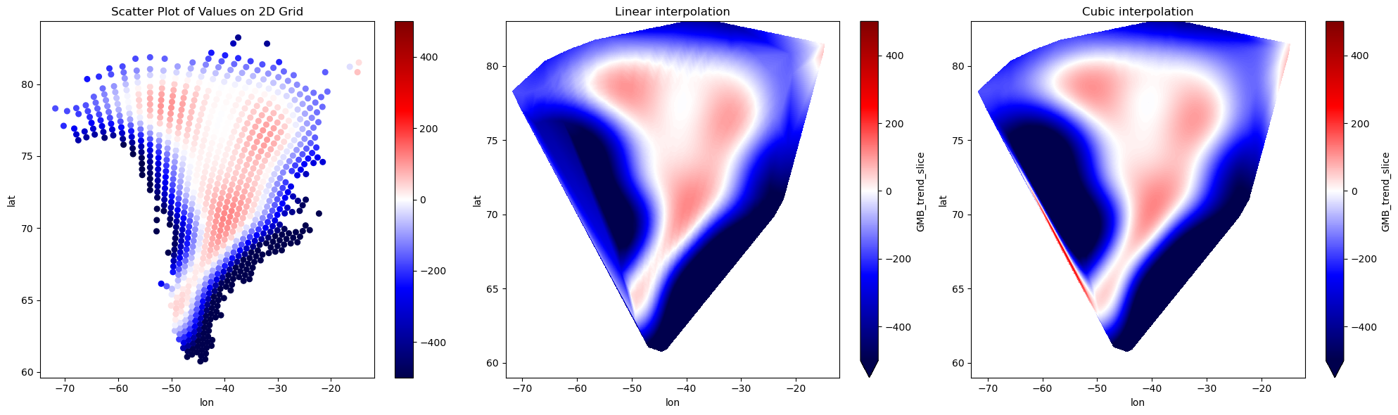
In this example, we will work with trend data of the Greenland ice sheet, which is provided as a set of spatial points over a given time range. We will apply several interpolation algorithms to fill the gaps between these points, ultimately converting the data into a raster format.

First we will open the data as usual.

ds = store.open_data("ESACCI-ICESHEETS_Greenland_GMB-2003-2016-v1.1.zarr")
ds

<xarray.Dataset> Size: 43kB
Dimensions:     (meas_ind: 901, time: 10)
Dimensions without coordinates: meas_ind, time
Data variables:
    GMB_trend   (meas_ind, time) float32 36kB dask.array<chunksize=(901, 10), meta=np.ndarray>
    end_time    (time) datetime64[ns] 80B dask.array<chunksize=(10,), meta=np.ndarray>
    latitude    (meas_ind) float32 4kB dask.array<chunksize=(901,), meta=np.ndarray>
    longitude   (meas_ind) float32 4kB dask.array<chunksize=(901,), meta=np.ndarray>
    start_time  (time) datetime64[ns] 80B dask.array<chunksize=(10,), meta=np.ndarray>
    t           (time) datetime64[ns] 80B dask.array<chunksize=(10,), meta=np.ndarray>
Attributes: (12/20)
    Institution:          DTU Space - Div. of Geodynamics
    Latitude_max:         83.23728
    Latitude_min:         60.73857
    Longitude_max:        -14.706720000000018
    Longitude_min:        -71.83566000000002
    Method:               GRACE GMB trend following Barletta et al. 2012
    ...                   ...
    grid_projection:      Geographical coordinates relative to WGS84
    netCDF_version:       NETCDF3_CLASSIC
    product_version:      1.2
    time_coverage_end:    2016-01-31
    time_coverage_start:  2003-01-01
    time_resolution:      5Y

xarray.Dataset

• Dimensions:
  • meas_ind: 901
  • time: 10
• Coordinates: (0)
• Data variables: (6)
  • GMB_trend
    (meas_ind, time)
    float32
    dask.array<chunksize=(901, 10), meta=np.ndarray>

    long_name :

    Mass trend for time span

    source :

    GRACE

    unit :

    mm water equivalent

    Array Chunk Bytes 35.20 kiB 35.20 kiB Shape (901, 10) (901, 10) Dask graph 1 chunks in 2 graph layers Data type float32 numpy.ndarray

  • end_time
    (time)
    datetime64[ns]
    dask.array<chunksize=(10,), meta=np.ndarray>

    long_name :

    End of time span

    title :

    Time

    Array Chunk Bytes 80 B 80 B Shape (10,) (10,) Dask graph 1 chunks in 2 graph layers Data type datetime64[ns] numpy.ndarray

  • latitude
    (meas_ind)
    float32
    dask.array<chunksize=(901,), meta=np.ndarray>

    long_name :

    latitude

    standard_name :

    latitude

    units :

    degrees_north

    Array Chunk Bytes 3.52 kiB 3.52 kiB Shape (901,) (901,) Dask graph 1 chunks in 2 graph layers Data type float32 numpy.ndarray

  • longitude
    (meas_ind)
    float32
    dask.array<chunksize=(901,), meta=np.ndarray>

    long_name :

    longitude

    standard_name :

    longitude

    units :

    degrees_east

    Array Chunk Bytes 3.52 kiB 3.52 kiB Shape (901,) (901,) Dask graph 1 chunks in 2 graph layers Data type float32 numpy.ndarray

  • start_time
    (time)
    datetime64[ns]
    dask.array<chunksize=(10,), meta=np.ndarray>

    long_name :

    Mean of time span

    title :

    Time

    Array Chunk Bytes 80 B 80 B Shape (10,) (10,) Dask graph 1 chunks in 2 graph layers Data type datetime64[ns] numpy.ndarray

  • t
    (time)
    datetime64[ns]
    dask.array<chunksize=(10,), meta=np.ndarray>

    long_name :

    Average time for time slice

    title :

    Time

    Array Chunk Bytes 80 B 80 B Shape (10,) (10,) Dask graph 1 chunks in 2 graph layers Data type datetime64[ns] numpy.ndarray

• Indexes: (0)
• Attributes: (20)

  Institution :

  DTU Space - Div. of Geodynamics

  Latitude_max :

  83.23728

  Latitude_min :

  60.73857

  Longitude_max :

  -14.706720000000018

  Longitude_min :

  -71.83566000000002

  Method :

  GRACE GMB trend following Barletta et al. 2012

  Project :

  Greenland ice sheet CCI.

  Source :

  GRACE

  Title :

  CCI GMB Greenland ice sheet

  Tracking_id :

  74eef7fd-f5c6-499b-a268-0621cdc0cbf6

  Units :

  Units used (mm water equivalent per year)

  abstract :

  This dataset provides the Gravitational Mass Balance (GMB) product derived from gravimetry data from the GRACE satellite instrument, by DTU Space. The data consists of two products: a mass change time series for the entire Greenland Ice Sheet and different drainage basins for the period April 2002 to June 2016; and mass trend grids for different 5-year periods between 2003 and 2016. This version (1.3) is derived from GRACE monthly solutions from the CSR RL06 product. The mass change time series contains the mass change (with respect to a chosen reference month) for all of the Greenland Ice Sheet and each individual drainage basin. For each month (defined by a decimal year) a mass change in Gt and its associated error (also in Gt) is provided. The mass trend grid product is given in units of mm water equivalent per year. Mass balance is an important variable to understand glacial thinning and ablation rates to enable mapping glacier area change. The time series allows the longer term comparison of trends whereas the mass trend grids provide a yearly snapshot which can be further analysed and compared across the data set. Basin definitions and further data descriptions can be found in the Algorithm Theoretical Baseline Document (ST-DTU-ESA-GISCCI-ATBD-001_v3.1.pdf) and Product Specification Document (ST-DTU-ESA-GISCCI-PSD_v2.2.pdf) which are provided on the Greenland Ice Sheet CCI project website. Citation: Barletta, V. R., Sorensen, L. S., and Forsberg, R.: Scatter of mass changes estimates at basin scale for Greenland and Antarctica, The Cryosphere, 7, 1411-1432, doi:10.5194/tc-7-1411-2013, 2013.

  catalogue_url :

  https://catalogue.ceda.ac.uk/uuid/ff4bfe39b7fe42fc993341d3cebdabb5

  date_created :

  Created Thu Jun 7 20:05:15 2018

  grid_projection :

  Geographical coordinates relative to WGS84

  netCDF_version :

  NETCDF3_CLASSIC

  product_version :

  1.2

  time_coverage_end :

  2016-01-31

  time_coverage_start :

  2003-01-01

  time_resolution :

  5Y

We define the final coordiates of the resired target raster and extract one time slice from the data set.

lon = np.arange(-73., -12., 0.02)
lat = np.arange(83., 59., -0.02)
grid_lon, grid_lat = np.meshgrid(lon, lat)
GMB_trend_slice = ds.GMB_trend.isel(time=0)

Now we can perform a 2D linear interpolation using scipy.interpolate.griddata.

gridded_data = interp.griddata(
    (ds.longitude, ds.latitude),
    GMB_trend_slice,
    (grid_lon, grid_lat),
    method='linear'
)
ds_linear = xr.Dataset(
    {'GMB_trend_slice': (['lat', 'lon'], gridded_data)},
    coords={'lon': lon, 'lat': lat}
)
ds_linear

<xarray.Dataset> Size: 29MB
Dimensions:          (lat: 1200, lon: 3050)
Coordinates:
  * lon              (lon) float64 24kB -73.0 -72.98 -72.96 ... -12.04 -12.02
  * lat              (lat) float64 10kB 83.0 82.98 82.96 ... 59.06 59.04 59.02
Data variables:
    GMB_trend_slice  (lat, lon) float64 29MB nan nan nan nan ... nan nan nan nan

xarray.Dataset

• Dimensions:
  • lat: 1200
  • lon: 3050
• Coordinates: (2)
  • lon
    (lon)
    float64
    -73.0 -72.98 ... -12.04 -12.02

    array([-73.  , -72.98, -72.96, ..., -12.06, -12.04, -12.02])

  • lat
    (lat)
    float64
    83.0 82.98 82.96 ... 59.04 59.02

    array([83.  , 82.98, 82.96, ..., 59.06, 59.04, 59.02])

• Data variables: (1)
  • GMB_trend_slice
    (lat, lon)
    float64
    nan nan nan nan ... nan nan nan nan

    array([[nan, nan, nan, ..., nan, nan, nan],
           [nan, nan, nan, ..., nan, nan, nan],
           [nan, nan, nan, ..., nan, nan, nan],
           ...,
           [nan, nan, nan, ..., nan, nan, nan],
           [nan, nan, nan, ..., nan, nan, nan],
           [nan, nan, nan, ..., nan, nan, nan]])

• Indexes: (2)
  • lon
    PandasIndex

    PandasIndex(Index([              -73.0,              -72.98,  -72.96000000000001,
            -72.94000000000001,  -72.92000000000002,  -72.90000000000002,
            -72.88000000000002,  -72.86000000000003,  -72.84000000000003,
            -72.82000000000004,
           ...
           -12.200000000012096,   -12.1800000000121, -12.160000000012104,
           -12.140000000012108, -12.120000000012112, -12.100000000012116,
            -12.08000000001212, -12.060000000012124, -12.040000000012128,
           -12.020000000012132],
          dtype='float64', name='lon', length=3050))

  • lat
    PandasIndex

    PandasIndex(Index([              83.0,              82.98,  82.96000000000001,
            82.94000000000001,  82.92000000000002,  82.90000000000002,
            82.88000000000002,  82.86000000000003,  82.84000000000003,
            82.82000000000004,
           ...
           59.200000000004735,  59.18000000000474,  59.16000000000474,
            59.14000000000475,  59.12000000000475, 59.100000000004755,
            59.08000000000476,  59.06000000000476,  59.04000000000477,
            59.02000000000477],
          dtype='float64', name='lat', length=1200))

• Attributes: (0)

The same approach can be applied using "cubic" as the interpolation method.

gridded_data = interp.griddata(
    (ds.longitude, ds.latitude),
    GMB_trend_slice,
    (grid_lon, grid_lat),
    method="cubic"
)
ds_cubic = xr.Dataset(
    {'GMB_trend_slice': (['lat', 'lon'], gridded_data)},
    coords={'lon': lon, 'lat': lat}
)
ds_cubic

<xarray.Dataset> Size: 29MB
Dimensions:          (lat: 1200, lon: 3050)
Coordinates:
  * lon              (lon) float64 24kB -73.0 -72.98 -72.96 ... -12.04 -12.02
  * lat              (lat) float64 10kB 83.0 82.98 82.96 ... 59.06 59.04 59.02
Data variables:
    GMB_trend_slice  (lat, lon) float64 29MB nan nan nan nan ... nan nan nan nan

xarray.Dataset

• Dimensions:
  • lat: 1200
  • lon: 3050
• Coordinates: (2)
  • lon
    (lon)
    float64
    -73.0 -72.98 ... -12.04 -12.02

    array([-73.  , -72.98, -72.96, ..., -12.06, -12.04, -12.02])

  • lat
    (lat)
    float64
    83.0 82.98 82.96 ... 59.04 59.02

    array([83.  , 82.98, 82.96, ..., 59.06, 59.04, 59.02])

• Data variables: (1)
  • GMB_trend_slice
    (lat, lon)
    float64
    nan nan nan nan ... nan nan nan nan

    array([[nan, nan, nan, ..., nan, nan, nan],
           [nan, nan, nan, ..., nan, nan, nan],
           [nan, nan, nan, ..., nan, nan, nan],
           ...,
           [nan, nan, nan, ..., nan, nan, nan],
           [nan, nan, nan, ..., nan, nan, nan],
           [nan, nan, nan, ..., nan, nan, nan]])

• Indexes: (2)
  • lon
    PandasIndex

    PandasIndex(Index([              -73.0,              -72.98,  -72.96000000000001,
            -72.94000000000001,  -72.92000000000002,  -72.90000000000002,
            -72.88000000000002,  -72.86000000000003,  -72.84000000000003,
            -72.82000000000004,
           ...
           -12.200000000012096,   -12.1800000000121, -12.160000000012104,
           -12.140000000012108, -12.120000000012112, -12.100000000012116,
            -12.08000000001212, -12.060000000012124, -12.040000000012128,
           -12.020000000012132],
          dtype='float64', name='lon', length=3050))

  • lat
    PandasIndex

    PandasIndex(Index([              83.0,              82.98,  82.96000000000001,
            82.94000000000001,  82.92000000000002,  82.90000000000002,
            82.88000000000002,  82.86000000000003,  82.84000000000003,
            82.82000000000004,
           ...
           59.200000000004735,  59.18000000000474,  59.16000000000474,
            59.14000000000475,  59.12000000000475, 59.100000000004755,
            59.08000000000476,  59.06000000000476,  59.04000000000477,
            59.02000000000477],
          dtype='float64', name='lat', length=1200))

• Attributes: (0)

Now, we can plot the results: the left plot shows the original points from the ESA CCI ice sheet trend dataset, the center plot displays the linear interpolation, and the right plot presents the cubic interpolation.

fig, ax = plt.subplots(1, 3, figsize=(20, 6))
scatter = ax[0].scatter(
    ds.longitude, ds.latitude, c=GMB_trend_slice, cmap='seismic', vmin=-500, vmax=500, s=30
)
ax[0].set_title('Scatter Plot of Values on 2D Grid')
ax[0].set_ylabel('lat')
ax[0].set_xlabel('lon')
fig.colorbar(scatter, ax=ax[0], orientation='vertical')
ds_linear.GMB_trend_slice.plot(ax=ax[1], vmin=-500, vmax=500, cmap='seismic')
ax[1].set_title('Linear interpolation')
ds_cubic.GMB_trend_slice.plot(ax=ax[2], vmin=-500, vmax=500, cmap='seismic')
ax[2].set_title('Cubic interpolation')

Text(0.5, 1.0, 'Cubic interpolation')

---

4.2.2.5.2. 2. Gap filling of a raster dataset

In this example, we will work with the soil moisture dataset, which is a 3d rastered dataset with gaps in it. We will show an example how to fill the gaps along the time axis for a time series and how to fill the pags in the 2d spatial domain.

First we will open the data as usual.

ds = store.open_data('ESACCI-SOILMOISTURE-L3S-SSMV-COMBINED-1978-2021-fv07.1.zarr')
ds

<xarray.Dataset> Size: 654GB
Dimensions:         (time: 15767, lat: 720, lon: 1440)
Coordinates:
  * lat             (lat) float64 6kB 89.88 89.62 89.38 ... -89.38 -89.62 -89.88
  * lon             (lon) float64 12kB -179.9 -179.6 -179.4 ... 179.6 179.9
  * time            (time) datetime64[ns] 126kB 1978-11-01 ... 2021-12-31
Data variables:
    dnflag          (time, lat, lon) float32 65GB dask.array<chunksize=(16, 720, 720), meta=np.ndarray>
    flag            (time, lat, lon) float32 65GB dask.array<chunksize=(16, 720, 720), meta=np.ndarray>
    freqbandID      (time, lat, lon) float32 65GB dask.array<chunksize=(16, 720, 720), meta=np.ndarray>
    mode            (time, lat, lon) float32 65GB dask.array<chunksize=(16, 720, 720), meta=np.ndarray>
    sensor          (time, lat, lon) float64 131GB dask.array<chunksize=(16, 720, 720), meta=np.ndarray>
    sm              (time, lat, lon) float32 65GB dask.array<chunksize=(16, 720, 720), meta=np.ndarray>
    sm_uncertainty  (time, lat, lon) float32 65GB dask.array<chunksize=(16, 720, 720), meta=np.ndarray>
    t0              (time, lat, lon) float64 131GB dask.array<chunksize=(16, 720, 720), meta=np.ndarray>
Attributes: (12/44)
    Conventions:                  CF-1.9
    cdm_data_type:                Grid
    comment:                      This dataset was produced with funding of t...
    contact:                      cci_sm_contact@eodc.eu
    creator_email:                cci_sm_developer@eodc.eu
    creator_name:                 Department of Geodesy and Geoinformation, V...
    ...                           ...
    time_coverage_end_product:    20211231T235959Z
    time_coverage_resolution:     P1D
    time_coverage_start:          1978-11-01 00:00:00
    time_coverage_start_product:  19781101T000000Z
    title:                        ESA CCI Surface Soil Moisture COMBINED acti...
    tracking_id:                  ad35798e-58e0-488f-b5b9-593874a47700

xarray.Dataset

• Dimensions:
  • time: 15767
  • lat: 720
  • lon: 1440
• Coordinates: (3)
  • lat
    (lat)
    float64
    89.88 89.62 89.38 ... -89.62 -89.88

    _CoordinateAxisType :

    Lat

    standard_name :

    latitude

    units :

    degrees_north

    valid_range :

    [-90.0, 90.0]

    array([ 89.875,  89.625,  89.375, ..., -89.375, -89.625, -89.875])

  • lon
    (lon)
    float64
    -179.9 -179.6 ... 179.6 179.9

    _CoordinateAxisType :

    Lon

    standard_name :

    longitude

    units :

    degrees_east

    valid_range :

    [-180.0, 180.0]

    array([-179.875, -179.625, -179.375, ...,  179.375,  179.625,  179.875])

  • time
    (time)
    datetime64[ns]
    1978-11-01 ... 2021-12-31

    array(['1978-11-01T00:00:00.000000000', '1978-11-02T00:00:00.000000000',
           '1978-11-03T00:00:00.000000000', ..., '2021-12-29T00:00:00.000000000',
           '2021-12-30T00:00:00.000000000', '2021-12-31T00:00:00.000000000'],
          dtype='datetime64[ns]')

• Data variables: (8)
  • dnflag
    (time, lat, lon)
    float32
    dask.array<chunksize=(16, 720, 720), meta=np.ndarray>

    _CoordinateAxes :

    time lat lon

    bit_meanings :

    ['NaN', 'day', 'night']

    bits :

    ['0b0', '0b1', '0b10']

    dtype :

    int8

    flag_meanings :

    ['NaN', 'day', 'night', 'day_night_combination']

    flag_values :

    [0, 1, 2, 3]

    long_name :

    Day / Night Flag

    valid_range :

    [0, 3]

    Array Chunk Bytes 60.90 GiB 31.64 MiB Shape (15767, 720, 1440) (16, 720, 720) Dask graph 1972 chunks in 2 graph layers Data type float32 numpy.ndarray

  • flag
    (time, lat, lon)
    float32
    dask.array<chunksize=(16, 720, 720), meta=np.ndarray>

    _CoordinateAxes :

    time lat lon

    bit_meanings :

    ['no_data_inconsistency_detected', 'snow_coverage_or_temperature_below_zero', 'dense_vegetation', 'others_no_convergence_in_the_model_thus_no_valid_sm_estimates', 'soil_moisture_value_exceeds_physical_boundary', 'weight_of_measurement_below_threshold', 'all_datasets_deemed_unreliable', 'barren_ground_advisory_flag', 'NaN']

    bits :

    ['0b0', '0b1', '0b10', '0b100', '0b1000', '0b10000', '0b100000', '0b1000000', '0b10000000']

    dtype :

    int16

    flag_meanings :

    ['no_data_inconsistency_detected', 'snow_coverage_or_temperature_below_zero', 'dense_vegetation', 'combination_of_flag_values_1_and_2', 'soil_moisture_value_exceeds_physical_boundary', 'combination_of_flag_values_1_and_8', 'combination_of_flag_values_2_and_8', 'barren_ground_advisory_flag', 'combination_of_flag_values_1_and_64', 'combination_of_flag_values_2_and_64', 'combination_of_flag_values_1_and_2_and_64', 'combination_of_flag_values_8_and_64', 'combination_of_flag_values_1_and_8_and_64', 'combination_of_flag_values_2_and_8_and_64', 'combination_of_flag_values_1_and_2_and_4_and_8_and_16_and_32_and_64']

    flag_values :

    [0, 1, 2, 3, 8, 9, 10, 64, 65, 66, 67, 72, 73, 74, 127]

    long_name :

    Flag

    standard_name :

    soil_moisture_content status_flag

    valid_range :

    [0, 255]

    Array Chunk Bytes 60.90 GiB 31.64 MiB Shape (15767, 720, 1440) (16, 720, 720) Dask graph 1972 chunks in 2 graph layers Data type float32 numpy.ndarray

  • freqbandID
    (time, lat, lon)
    float32
    dask.array<chunksize=(16, 720, 720), meta=np.ndarray>

    _CoordinateAxes :

    time lat lon

    bit_meanings :

    ['NaN', 'L14', 'C53', 'C66', 'C68', 'C69', 'C73', 'X107', 'K194', 'MODEL']

    bits :

    ['0b0', '0b1', '0b10', '0b100', '0b1000', '0b10000', '0b100000', '0b1000000', '0b10000000', '0b100000000']

    dtype :

    int16

    flag_meanings :

    ['NaN', 'C66', 'X107', 'C66+X107']

    flag_values :

    [0, 4, 64, 68]

    long_name :

    Frequency Band Identification

    valid_range :

    [0, 511]

    Array Chunk Bytes 60.90 GiB 31.64 MiB Shape (15767, 720, 1440) (16, 720, 720) Dask graph 1972 chunks in 2 graph layers Data type float32 numpy.ndarray

  • mode
    (time, lat, lon)
    float32
    dask.array<chunksize=(16, 720, 720), meta=np.ndarray>

    _CoordinateAxes :

    time lat lon

    bit_meanings :

    ['NaN', 'ascending', 'descending']

    bits :

    ['0b0', '0b1', '0b10']

    dtype :

    int8

    flag_meanings :

    ['NaN', 'ascending', 'descending', 'ascending_descending_combination']

    flag_values :

    [0, 1, 2, 3]

    long_name :

    Satellite Mode

    valid_range :

    [0, 3]

    Array Chunk Bytes 60.90 GiB 31.64 MiB Shape (15767, 720, 1440) (16, 720, 720) Dask graph 1972 chunks in 2 graph layers Data type float32 numpy.ndarray

  • sensor
    (time, lat, lon)
    float64
    dask.array<chunksize=(16, 720, 720), meta=np.ndarray>

    _CoordinateAxes :

    time lat lon

    bit_meanings :

    ['NaN', 'SMMR', 'SSMI', 'TMI', 'AMSRE', 'WindSat', 'AMSR2', 'SMOS', 'AMIWS', 'ASCATA', 'ASCATB', 'SMAP', 'MODEL', 'GPM', 'FY3B', 'FY3D', 'ASCATC', 'FY3C']

    bits :

    ['0b0', '0b1', '0b10', '0b100', '0b1000', '0b10000', '0b100000', '0b1000000', '0b10000000', '0b100000000', '0b1000000000', '0b10000000000', '0b100000000000', '0b1000000000000', '0b10000000000000', '0b100000000000000', '0b1000000000000000', '0b10000000000000000']

    dtype :

    int32

    flag_meanings :

    ['NaN', 'SMMR']

    flag_values :

    [0, 1]

    long_name :

    Sensor

    valid_range :

    [0, 131071]

    Array Chunk Bytes 121.80 GiB 63.28 MiB Shape (15767, 720, 1440) (16, 720, 720) Dask graph 1972 chunks in 2 graph layers Data type float64 numpy.ndarray

  • sm
    (time, lat, lon)
    float32
    dask.array<chunksize=(16, 720, 720), meta=np.ndarray>

    _CoordinateAxes :

    time lat lon

    ancillary_variables :

    sm_uncertainty flag t0

    dtype :

    float32

    long_name :

    Volumetric Soil Moisture

    standard_name :

    soil_moisture_content

    units :

    m3 m-3

    valid_range :

    [0.0, 1.0]

    Array Chunk Bytes 60.90 GiB 31.64 MiB Shape (15767, 720, 1440) (16, 720, 720) Dask graph 1972 chunks in 2 graph layers Data type float32 numpy.ndarray

  • sm_uncertainty
    (time, lat, lon)
    float32
    dask.array<chunksize=(16, 720, 720), meta=np.ndarray>

    _CoordinateAxes :

    time lat lon

    dtype :

    float32

    long_name :

    Volumetric Soil Moisture Uncertainty

    standard_name :

    soil_moisture_content standard_error

    units :

    m3 m-3

    valid_range :

    [0.0, 1.0]

    Array Chunk Bytes 60.90 GiB 31.64 MiB Shape (15767, 720, 1440) (16, 720, 720) Dask graph 1972 chunks in 2 graph layers Data type float32 numpy.ndarray

  • t0
    (time, lat, lon)
    float64
    dask.array<chunksize=(16, 720, 720), meta=np.ndarray>

    _CoordinateAxes :

    time lat lon

    dtype :

    float64

    long_name :

    Observation Timestamp

    units :

    days after 1970-01-01 00:00:00 UTC

    valid_range :

    [3225.0, 3227.0]

    Array Chunk Bytes 121.80 GiB 63.28 MiB Shape (15767, 720, 1440) (16, 720, 720) Dask graph 1972 chunks in 2 graph layers Data type float64 numpy.ndarray

• Indexes: (3)
  • lat
    PandasIndex

    PandasIndex(Index([ 89.875,  89.625,  89.375,  89.125,  88.875,  88.625,  88.375,  88.125,
            87.875,  87.625,
           ...
           -87.625, -87.875, -88.125, -88.375, -88.625, -88.875, -89.125, -89.375,
           -89.625, -89.875],
          dtype='float64', name='lat', length=720))

  • lon
    PandasIndex

    PandasIndex(Index([-179.875, -179.625, -179.375, -179.125, -178.875, -178.625, -178.375,
           -178.125, -177.875, -177.625,
           ...
            177.625,  177.875,  178.125,  178.375,  178.625,  178.875,  179.125,
            179.375,  179.625,  179.875],
          dtype='float64', name='lon', length=1440))

  • time
    PandasIndex

    PandasIndex(DatetimeIndex(['1978-11-01', '1978-11-02', '1978-11-03', '1978-11-04',
                   '1978-11-05', '1978-11-06', '1978-11-07', '1978-11-08',
                   '1978-11-09', '1978-11-10',
                   ...
                   '2021-12-22', '2021-12-23', '2021-12-24', '2021-12-25',
                   '2021-12-26', '2021-12-27', '2021-12-28', '2021-12-29',
                   '2021-12-30', '2021-12-31'],
                  dtype='datetime64[ns]', name='time', length=15767, freq=None))

• Attributes: (44)

  Conventions :

  CF-1.9

  cdm_data_type :

  Grid

  comment :

  This dataset was produced with funding of the ESA CCI+ Soil Moisture project; ESRIN Contract No: 4000126684/19/I-NB

  contact :

  cci_sm_contact@eodc.eu

  creator_email :

  cci_sm_developer@eodc.eu

  creator_name :

  Department of Geodesy and Geoinformation, Vienna University of Technology

  creator_url :

  https://climers.geo.tuwien.ac.at/

  date_created :

  File created: 2022-04-06 12:31:39.526359

  geospatial_lat_max :

  90.0

  geospatial_lat_min :

  -90.0

  geospatial_lat_resolution :

  0.25 degree

  geospatial_lat_units :

  degrees_north

  geospatial_lon_max :

  180.0

  geospatial_lon_min :

  -180.0

  geospatial_lon_resolution :

  0.25 degree

  geospatial_lon_units :

  degrees_east

  geospatial_vertical_max :

  0.0

  geospatial_vertical_min :

  0.0

  history :

  2022-04-06 12:29:35 - product produced 2023-08-09 17:33:51 - converted by nc2zarr, version 1.1.2.dev0

  id :

  ESACCI-SOILMOISTURE-L3S-SSMV-COMBINED-20211231000000-fv07.1.nc

  institution :

  TU Wien (AUT); VanderSat B.V. (NL)

  key_variables :

  sm

  keywords :

  soil moisture, soil water content, microwave remote sensing, active, passive, combined, climate data record

  keywords_vocabulary :

  NASA Global Change Master Directory (GCMD) Science Keywords

  license :

  Data use is free and open for all registered users.

  naming_authority :

  TU Wien

  platform :

  Nimbus 7, DMSP, TRMM, AQUA, Coriolis, GCOM-W1, MIRAS, SMAP, GPM, FengYun-3B, FengYun-3C, FengYun-3D; ERS-1, ERS-2, METOP-A, METOP-B

  processing_level :

  Quality-controlled, super-collocated (L3S) Satellite Soil Moisture (SM) data from multiple sensors

  product_version :

  v07.1

  project :

  Climate Change Initiative - European Space Agency

  references :

  http://www.esa-soilmoisture-cci.org; Dorigo, W.A., Wagner, W., Albergel, C., Albrecht, F., Balsamo, G., Brocca, L., Chung, D., Ertl, M., Forkel, M., Gruber, A., Haas, E., Hamer, D. P. Hirschi, M., Ikonen, J., De Jeu, R. Kidd, R. Lahoz, W., Liu, Y.Y., Miralles, D., Lecomte, P. (2017) ESA CCI Soil Moisture for improved Earth system understanding: State-of-the art and future directions. In Remote Sensing of Environment, 2017, ISSN 0034-4257, https://doi.org/10.1016/j.rse.2017.07.001; Gruber, A., Scanlon, T., van der Schalie, R., Wagner, W., Dorigo, W. (2019) Evolution of the ESA CCI Soil Moisture Climate Data Records and their underlying merging methodology. Earth System Science Data 11, 717-739, https://doi.org/10.5194/essd-11-717-2019; Gruber, A., Dorigo, W. A., Crow, W., Wagner W. (2017). Triple Collocation-Based Merging of Satellite Soil Moisture Retrievals. IEEE Transactions on Geoscience and Remote Sensing. PP. 1-13. https://doi.org/10.1109/TGRS.2017.2734070

  sensor :

  SMMR, SSM/I, TMI, AMSR-E, WindSat, AMSR2, SMOS, SMAP_radiometer, GMI, VIRR-3B, VIRR-3C, VIRR-3D; AMI-WS, ASCAT-A, ASCAT-B, ASCAT-C

  source :

  WARP 5.5R1.1/AMI-WS/ERS12 Level 2 Soil Moisture; WARP 5.4R1.0/AMI-WS/ERS2 Level 2 Soil Moisture; H115: Metop ASCAT Surface Soil Moisture Climate Data Record v5 12.5 km sampling, DOI: 10.15770/EUM_SAF_H_0006; H116: Metop ASCAT Surface Soil Moisture Climate Data Record v5 Extension 12.5 km sampling; H115: Metop ASCAT Surface Soil Moisture Climate Data Record v5 12.5 km sampling, DOI: 10.15770/EUM_SAF_H_0006; H116: Metop ASCAT Surface Soil Moisture Climate Data Record v5 Extension 12.5 km sampling; H115: Metop ASCAT Surface Soil Moisture Climate Data Record v5 12.5 km sampling, DOI: 10.15770/EUM_SAF_H_0006; H116: Metop ASCAT Surface Soil Moisture Climate Data Record v5 Extension 12.5 km sampling;; LPRMv7/SMMR/Nimbus 7 L3 Surface Soil Moisture, Ancillary Params, and quality flags; LPRMv7/SSMI/F08, F11, F13 DMSP L3 Surface Soil Moisture, Ancillary Params, and quality flags; LPRMv7/TMI/TRMM L2 Surface Soil Moisture, Ancillary Params, and QC; LPRMv7/AMSR-E/Aqua L2B Surface Soil Moisture, Ancillary Params, and QC; LPRMv7/WINDSAT/CORIOLIS L2 Surface Soil Moisture, Ancillary Params, and QC; LPRMv7/AMSR2/GCOM-W1 L3 Surface Soil Moisture, Ancillary Params; LPRMv7/SMOS/MIRAS L3 Surface Soil Moisture, CATDS Level 3 Brightness Temperatures (L3TB) version 300 RE03 & RE04; LPRMv7/SMAP_radiometer/SMAP L2 Surface Soil Moisture, Ancillary Params, and QC; LPRMv7/GMI/GPM L3 Surface Soil Moisture, Ancillary Params, and quality flags; LPRMv7/VIRR/FengYun-3B L3 Surface Soil Moisture, Ancillary Params, and quality flags; LPRMv7/VIRR/FengYun-3C L3 Surface Soil Moisture, Ancillary Params, and quality flags; LPRMv7/VIRR/FengYun-3D L3 Surface Soil Moisture, Ancillary Params, and quality flags;;

  spatial_resolution :

  25km

  standard_name_vocabulary :

  CF Standard Name Table v77

  summary :

  This dataset was produced with funding of the ESA CCI+ Soil Moisture project; ESRIN Contract No: 4000126684/19/I-NB

  time_coverage_duration :

  P43Y

  time_coverage_end :

  2021-12-31 00:00:00

  time_coverage_end_product :

  20211231T235959Z

  time_coverage_resolution :

  P1D

  time_coverage_start :

  1978-11-01 00:00:00

  time_coverage_start_product :

  19781101T000000Z

  title :

  ESA CCI Surface Soil Moisture COMBINED active+passive Product

  tracking_id :

  ad35798e-58e0-488f-b5b9-593874a47700

4.2.2.5.2.1. Gap filling along the time axis

For this, we create a small function that removes all NaN values and then performs interpolation to the original time axis using xarray.Dataset.interp().

def fill_temporal_gaps(ds, method="linear"):
    new_times = ds_ts.time
    ds_nonans = ds_ts.dropna(dim="time")
    return ds_nonans.interp(time=new_times, method=method)

We will apply this gap-filling method to one year of the dataset as an example. To do this, we subset the dataset and select the year 2000.

ds_ts = ds.sel(lat=20, lon=20, method="nearest")
ds_ts = ds_ts.sel(time=slice('2000-01-01 00:00:00', '2001-01-01 00:00:00'))
ds_ts

<xarray.Dataset> Size: 18kB
Dimensions:         (time: 367)
Coordinates:
    lat             float64 8B 20.12
    lon             float64 8B 20.12
  * time            (time) datetime64[ns] 3kB 2000-01-01 ... 2001-01-01
Data variables:
    dnflag          (time) float32 1kB dask.array<chunksize=(13,), meta=np.ndarray>
    flag            (time) float32 1kB dask.array<chunksize=(13,), meta=np.ndarray>
    freqbandID      (time) float32 1kB dask.array<chunksize=(13,), meta=np.ndarray>
    mode            (time) float32 1kB dask.array<chunksize=(13,), meta=np.ndarray>
    sensor          (time) float64 3kB dask.array<chunksize=(13,), meta=np.ndarray>
    sm              (time) float32 1kB dask.array<chunksize=(13,), meta=np.ndarray>
    sm_uncertainty  (time) float32 1kB dask.array<chunksize=(13,), meta=np.ndarray>
    t0              (time) float64 3kB dask.array<chunksize=(13,), meta=np.ndarray>
Attributes: (12/44)
    Conventions:                  CF-1.9
    cdm_data_type:                Grid
    comment:                      This dataset was produced with funding of t...
    contact:                      cci_sm_contact@eodc.eu
    creator_email:                cci_sm_developer@eodc.eu
    creator_name:                 Department of Geodesy and Geoinformation, V...
    ...                           ...
    time_coverage_end_product:    20211231T235959Z
    time_coverage_resolution:     P1D
    time_coverage_start:          1978-11-01 00:00:00
    time_coverage_start_product:  19781101T000000Z
    title:                        ESA CCI Surface Soil Moisture COMBINED acti...
    tracking_id:                  ad35798e-58e0-488f-b5b9-593874a47700

xarray.Dataset

• Dimensions:
  • time: 367
• Coordinates: (3)
  • lat
    ()
    float64
    20.12

    _CoordinateAxisType :

    Lat

    standard_name :

    latitude

    units :

    degrees_north

    valid_range :

    [-90.0, 90.0]

    array(20.125)

  • lon
    ()
    float64
    20.12

    _CoordinateAxisType :

    Lon

    standard_name :

    longitude

    units :

    degrees_east

    valid_range :

    [-180.0, 180.0]

    array(20.125)

  • time
    (time)
    datetime64[ns]
    2000-01-01 ... 2001-01-01

    array(['2000-01-01T00:00:00.000000000', '2000-01-02T00:00:00.000000000',
           '2000-01-03T00:00:00.000000000', ..., '2000-12-30T00:00:00.000000000',
           '2000-12-31T00:00:00.000000000', '2001-01-01T00:00:00.000000000'],
          dtype='datetime64[ns]')

• Data variables: (8)
  • dnflag
    (time)
    float32
    dask.array<chunksize=(13,), meta=np.ndarray>

    _CoordinateAxes :

    time lat lon

    bit_meanings :

    ['NaN', 'day', 'night']

    bits :

    ['0b0', '0b1', '0b10']

    dtype :

    int8

    flag_meanings :

    ['NaN', 'day', 'night', 'day_night_combination']

    flag_values :

    [0, 1, 2, 3]

    long_name :

    Day / Night Flag

    valid_range :

    [0, 3]

    Array Chunk Bytes 1.43 kiB 64 B Shape (367,) (16,) Dask graph 24 chunks in 4 graph layers Data type float32 numpy.ndarray

  • flag
    (time)
    float32
    dask.array<chunksize=(13,), meta=np.ndarray>

    _CoordinateAxes :

    time lat lon

    bit_meanings :

    ['no_data_inconsistency_detected', 'snow_coverage_or_temperature_below_zero', 'dense_vegetation', 'others_no_convergence_in_the_model_thus_no_valid_sm_estimates', 'soil_moisture_value_exceeds_physical_boundary', 'weight_of_measurement_below_threshold', 'all_datasets_deemed_unreliable', 'barren_ground_advisory_flag', 'NaN']

    bits :

    ['0b0', '0b1', '0b10', '0b100', '0b1000', '0b10000', '0b100000', '0b1000000', '0b10000000']

    dtype :

    int16

    flag_meanings :

    ['no_data_inconsistency_detected', 'snow_coverage_or_temperature_below_zero', 'dense_vegetation', 'combination_of_flag_values_1_and_2', 'soil_moisture_value_exceeds_physical_boundary', 'combination_of_flag_values_1_and_8', 'combination_of_flag_values_2_and_8', 'barren_ground_advisory_flag', 'combination_of_flag_values_1_and_64', 'combination_of_flag_values_2_and_64', 'combination_of_flag_values_1_and_2_and_64', 'combination_of_flag_values_8_and_64', 'combination_of_flag_values_1_and_8_and_64', 'combination_of_flag_values_2_and_8_and_64', 'combination_of_flag_values_1_and_2_and_4_and_8_and_16_and_32_and_64']

    flag_values :

    [0, 1, 2, 3, 8, 9, 10, 64, 65, 66, 67, 72, 73, 74, 127]

    long_name :

    Flag

    standard_name :

    soil_moisture_content status_flag

    valid_range :

    [0, 255]

    Array Chunk Bytes 1.43 kiB 64 B Shape (367,) (16,) Dask graph 24 chunks in 4 graph layers Data type float32 numpy.ndarray

  • freqbandID
    (time)
    float32
    dask.array<chunksize=(13,), meta=np.ndarray>

    _CoordinateAxes :

    time lat lon

    bit_meanings :

    ['NaN', 'L14', 'C53', 'C66', 'C68', 'C69', 'C73', 'X107', 'K194', 'MODEL']

    bits :

    ['0b0', '0b1', '0b10', '0b100', '0b1000', '0b10000', '0b100000', '0b1000000', '0b10000000', '0b100000000']

    dtype :

    int16

    flag_meanings :

    ['NaN', 'C66', 'X107', 'C66+X107']

    flag_values :

    [0, 4, 64, 68]

    long_name :

    Frequency Band Identification

    valid_range :

    [0, 511]

    Array Chunk Bytes 1.43 kiB 64 B Shape (367,) (16,) Dask graph 24 chunks in 4 graph layers Data type float32 numpy.ndarray

  • mode
    (time)
    float32
    dask.array<chunksize=(13,), meta=np.ndarray>

    _CoordinateAxes :

    time lat lon

    bit_meanings :

    ['NaN', 'ascending', 'descending']

    bits :

    ['0b0', '0b1', '0b10']

    dtype :

    int8

    flag_meanings :

    ['NaN', 'ascending', 'descending', 'ascending_descending_combination']

    flag_values :

    [0, 1, 2, 3]

    long_name :

    Satellite Mode

    valid_range :

    [0, 3]

    Array Chunk Bytes 1.43 kiB 64 B Shape (367,) (16,) Dask graph 24 chunks in 4 graph layers Data type float32 numpy.ndarray

  • sensor
    (time)
    float64
    dask.array<chunksize=(13,), meta=np.ndarray>

    _CoordinateAxes :

    time lat lon

    bit_meanings :

    ['NaN', 'SMMR', 'SSMI', 'TMI', 'AMSRE', 'WindSat', 'AMSR2', 'SMOS', 'AMIWS', 'ASCATA', 'ASCATB', 'SMAP', 'MODEL', 'GPM', 'FY3B', 'FY3D', 'ASCATC', 'FY3C']

    bits :

    ['0b0', '0b1', '0b10', '0b100', '0b1000', '0b10000', '0b100000', '0b1000000', '0b10000000', '0b100000000', '0b1000000000', '0b10000000000', '0b100000000000', '0b1000000000000', '0b10000000000000', '0b100000000000000', '0b1000000000000000', '0b10000000000000000']

    dtype :

    int32

    flag_meanings :

    ['NaN', 'SMMR']

    flag_values :

    [0, 1]

    long_name :

    Sensor

    valid_range :

    [0, 131071]

    Array Chunk Bytes 2.87 kiB 128 B Shape (367,) (16,) Dask graph 24 chunks in 4 graph layers Data type float64 numpy.ndarray

  • sm
    (time)
    float32
    dask.array<chunksize=(13,), meta=np.ndarray>

    _CoordinateAxes :

    time lat lon

    ancillary_variables :

    sm_uncertainty flag t0

    dtype :

    float32

    long_name :

    Volumetric Soil Moisture

    standard_name :

    soil_moisture_content

    units :

    m3 m-3

    valid_range :

    [0.0, 1.0]

    Array Chunk Bytes 1.43 kiB 64 B Shape (367,) (16,) Dask graph 24 chunks in 4 graph layers Data type float32 numpy.ndarray

  • sm_uncertainty
    (time)
    float32
    dask.array<chunksize=(13,), meta=np.ndarray>

    _CoordinateAxes :

    time lat lon

    dtype :

    float32

    long_name :

    Volumetric Soil Moisture Uncertainty

    standard_name :

    soil_moisture_content standard_error

    units :

    m3 m-3

    valid_range :

    [0.0, 1.0]

    Array Chunk Bytes 1.43 kiB 64 B Shape (367,) (16,) Dask graph 24 chunks in 4 graph layers Data type float32 numpy.ndarray

  • t0
    (time)
    float64
    dask.array<chunksize=(13,), meta=np.ndarray>

    _CoordinateAxes :

    time lat lon

    dtype :

    float64

    long_name :

    Observation Timestamp

    units :

    days after 1970-01-01 00:00:00 UTC

    valid_range :

    [3225.0, 3227.0]

    Array Chunk Bytes 2.87 kiB 128 B Shape (367,) (16,) Dask graph 24 chunks in 4 graph layers Data type float64 numpy.ndarray

• Indexes: (1)
  • time
    PandasIndex

    PandasIndex(DatetimeIndex(['2000-01-01', '2000-01-02', '2000-01-03', '2000-01-04',
                   '2000-01-05', '2000-01-06', '2000-01-07', '2000-01-08',
                   '2000-01-09', '2000-01-10',
                   ...
                   '2000-12-23', '2000-12-24', '2000-12-25', '2000-12-26',
                   '2000-12-27', '2000-12-28', '2000-12-29', '2000-12-30',
                   '2000-12-31', '2001-01-01'],
                  dtype='datetime64[ns]', name='time', length=367, freq=None))

• Attributes: (44)

  Conventions :

  CF-1.9

  cdm_data_type :

  Grid

  comment :

  This dataset was produced with funding of the ESA CCI+ Soil Moisture project; ESRIN Contract No: 4000126684/19/I-NB

  contact :

  cci_sm_contact@eodc.eu

  creator_email :

  cci_sm_developer@eodc.eu

  creator_name :

  Department of Geodesy and Geoinformation, Vienna University of Technology

  creator_url :

  https://climers.geo.tuwien.ac.at/

  date_created :

  File created: 2022-04-06 12:31:39.526359

  geospatial_lat_max :

  90.0

  geospatial_lat_min :

  -90.0

  geospatial_lat_resolution :

  0.25 degree

  geospatial_lat_units :

  degrees_north

  geospatial_lon_max :

  180.0

  geospatial_lon_min :

  -180.0

  geospatial_lon_resolution :

  0.25 degree

  geospatial_lon_units :

  degrees_east

  geospatial_vertical_max :

  0.0

  geospatial_vertical_min :

  0.0

  history :

  2022-04-06 12:29:35 - product produced 2023-08-09 17:33:51 - converted by nc2zarr, version 1.1.2.dev0

  id :

  ESACCI-SOILMOISTURE-L3S-SSMV-COMBINED-20211231000000-fv07.1.nc

  institution :

  TU Wien (AUT); VanderSat B.V. (NL)

  key_variables :

  sm

  keywords :

  soil moisture, soil water content, microwave remote sensing, active, passive, combined, climate data record

  keywords_vocabulary :

  NASA Global Change Master Directory (GCMD) Science Keywords

  license :

  Data use is free and open for all registered users.

  naming_authority :

  TU Wien

  platform :

  Nimbus 7, DMSP, TRMM, AQUA, Coriolis, GCOM-W1, MIRAS, SMAP, GPM, FengYun-3B, FengYun-3C, FengYun-3D; ERS-1, ERS-2, METOP-A, METOP-B

  processing_level :

  Quality-controlled, super-collocated (L3S) Satellite Soil Moisture (SM) data from multiple sensors

  product_version :

  v07.1

  project :

  Climate Change Initiative - European Space Agency

  references :

  http://www.esa-soilmoisture-cci.org; Dorigo, W.A., Wagner, W., Albergel, C., Albrecht, F., Balsamo, G., Brocca, L., Chung, D., Ertl, M., Forkel, M., Gruber, A., Haas, E., Hamer, D. P. Hirschi, M., Ikonen, J., De Jeu, R. Kidd, R. Lahoz, W., Liu, Y.Y., Miralles, D., Lecomte, P. (2017) ESA CCI Soil Moisture for improved Earth system understanding: State-of-the art and future directions. In Remote Sensing of Environment, 2017, ISSN 0034-4257, https://doi.org/10.1016/j.rse.2017.07.001; Gruber, A., Scanlon, T., van der Schalie, R., Wagner, W., Dorigo, W. (2019) Evolution of the ESA CCI Soil Moisture Climate Data Records and their underlying merging methodology. Earth System Science Data 11, 717-739, https://doi.org/10.5194/essd-11-717-2019; Gruber, A., Dorigo, W. A., Crow, W., Wagner W. (2017). Triple Collocation-Based Merging of Satellite Soil Moisture Retrievals. IEEE Transactions on Geoscience and Remote Sensing. PP. 1-13. https://doi.org/10.1109/TGRS.2017.2734070

  sensor :

  SMMR, SSM/I, TMI, AMSR-E, WindSat, AMSR2, SMOS, SMAP_radiometer, GMI, VIRR-3B, VIRR-3C, VIRR-3D; AMI-WS, ASCAT-A, ASCAT-B, ASCAT-C

  source :

  WARP 5.5R1.1/AMI-WS/ERS12 Level 2 Soil Moisture; WARP 5.4R1.0/AMI-WS/ERS2 Level 2 Soil Moisture; H115: Metop ASCAT Surface Soil Moisture Climate Data Record v5 12.5 km sampling, DOI: 10.15770/EUM_SAF_H_0006; H116: Metop ASCAT Surface Soil Moisture Climate Data Record v5 Extension 12.5 km sampling; H115: Metop ASCAT Surface Soil Moisture Climate Data Record v5 12.5 km sampling, DOI: 10.15770/EUM_SAF_H_0006; H116: Metop ASCAT Surface Soil Moisture Climate Data Record v5 Extension 12.5 km sampling; H115: Metop ASCAT Surface Soil Moisture Climate Data Record v5 12.5 km sampling, DOI: 10.15770/EUM_SAF_H_0006; H116: Metop ASCAT Surface Soil Moisture Climate Data Record v5 Extension 12.5 km sampling;; LPRMv7/SMMR/Nimbus 7 L3 Surface Soil Moisture, Ancillary Params, and quality flags; LPRMv7/SSMI/F08, F11, F13 DMSP L3 Surface Soil Moisture, Ancillary Params, and quality flags; LPRMv7/TMI/TRMM L2 Surface Soil Moisture, Ancillary Params, and QC; LPRMv7/AMSR-E/Aqua L2B Surface Soil Moisture, Ancillary Params, and QC; LPRMv7/WINDSAT/CORIOLIS L2 Surface Soil Moisture, Ancillary Params, and QC; LPRMv7/AMSR2/GCOM-W1 L3 Surface Soil Moisture, Ancillary Params; LPRMv7/SMOS/MIRAS L3 Surface Soil Moisture, CATDS Level 3 Brightness Temperatures (L3TB) version 300 RE03 & RE04; LPRMv7/SMAP_radiometer/SMAP L2 Surface Soil Moisture, Ancillary Params, and QC; LPRMv7/GMI/GPM L3 Surface Soil Moisture, Ancillary Params, and quality flags; LPRMv7/VIRR/FengYun-3B L3 Surface Soil Moisture, Ancillary Params, and quality flags; LPRMv7/VIRR/FengYun-3C L3 Surface Soil Moisture, Ancillary Params, and quality flags; LPRMv7/VIRR/FengYun-3D L3 Surface Soil Moisture, Ancillary Params, and quality flags;;

  spatial_resolution :

  25km

  standard_name_vocabulary :

  CF Standard Name Table v77

  summary :

  This dataset was produced with funding of the ESA CCI+ Soil Moisture project; ESRIN Contract No: 4000126684/19/I-NB

  time_coverage_duration :

  P43Y

  time_coverage_end :

  2021-12-31 00:00:00

  time_coverage_end_product :

  20211231T235959Z

  time_coverage_resolution :

  P1D

  time_coverage_start :

  1978-11-01 00:00:00

  time_coverage_start_product :

  19781101T000000Z

  title :

  ESA CCI Surface Soil Moisture COMBINED active+passive Product

  tracking_id :

  ad35798e-58e0-488f-b5b9-593874a47700

Next, we apply the gap-filling method to the selected sample.

ds_ts_gap_fill = fill_temporal_gaps(ds_ts)
ds_ts_gap_fill

<xarray.Dataset> Size: 18kB
Dimensions:         (time: 367)
Coordinates:
    lat             float64 8B 20.12
    lon             float64 8B 20.12
  * time            (time) datetime64[ns] 3kB 2000-01-01 ... 2001-01-01
Data variables:
    dnflag          (time) float32 1kB dask.array<chunksize=(367,), meta=np.ndarray>
    flag            (time) float32 1kB dask.array<chunksize=(367,), meta=np.ndarray>
    freqbandID      (time) float32 1kB dask.array<chunksize=(367,), meta=np.ndarray>
    mode            (time) float32 1kB dask.array<chunksize=(367,), meta=np.ndarray>
    sensor          (time) float64 3kB dask.array<chunksize=(367,), meta=np.ndarray>
    sm              (time) float32 1kB dask.array<chunksize=(367,), meta=np.ndarray>
    sm_uncertainty  (time) float32 1kB dask.array<chunksize=(367,), meta=np.ndarray>
    t0              (time) float64 3kB dask.array<chunksize=(367,), meta=np.ndarray>
Attributes: (12/44)
    Conventions:                  CF-1.9
    cdm_data_type:                Grid
    comment:                      This dataset was produced with funding of t...
    contact:                      cci_sm_contact@eodc.eu
    creator_email:                cci_sm_developer@eodc.eu
    creator_name:                 Department of Geodesy and Geoinformation, V...
    ...                           ...
    time_coverage_end_product:    20211231T235959Z
    time_coverage_resolution:     P1D
    time_coverage_start:          1978-11-01 00:00:00
    time_coverage_start_product:  19781101T000000Z
    title:                        ESA CCI Surface Soil Moisture COMBINED acti...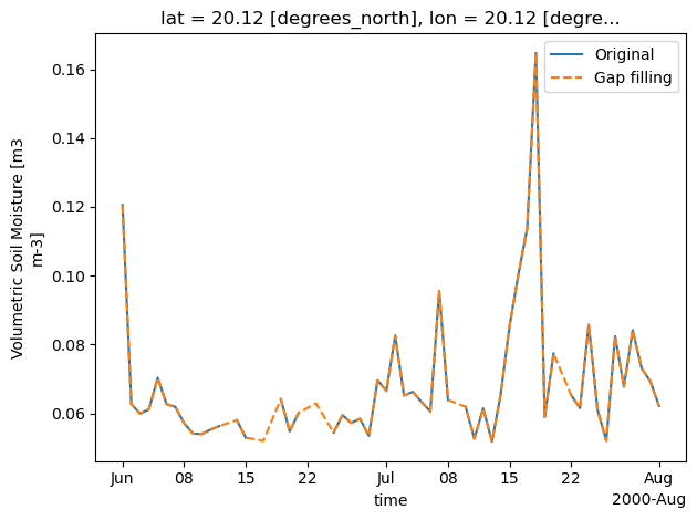
    tracking_id:                  ad35798e-58e0-488f-b5b9-593874a47700

xarray.Dataset

• Dimensions:
  • time: 367
• Coordinates: (3)
  • lat
    ()
    float64
    20.12

    _CoordinateAxisType :

    Lat

    standard_name :

    latitude

    units :

    degrees_north

    valid_range :

    [-90.0, 90.0]

    array(20.125)

  • lon
    ()
    float64
    20.12

    _CoordinateAxisType :

    Lon

    standard_name :

    longitude

    units :

    degrees_east

    valid_range :

    [-180.0, 180.0]

    array(20.125)

  • time
    (time)
    datetime64[ns]
    2000-01-01 ... 2001-01-01

    array(['2000-01-01T00:00:00.000000000', '2000-01-02T00:00:00.000000000',
           '2000-01-03T00:00:00.000000000', ..., '2000-12-30T00:00:00.000000000',
           '2000-12-31T00:00:00.000000000', '2001-01-01T00:00:00.000000000'],
          dtype='datetime64[ns]')

• Data variables: (8)
  • dnflag
    (time)
    float32
    dask.array<chunksize=(367,), meta=np.ndarray>

    _CoordinateAxes :

    time lat lon

    bit_meanings :

    ['NaN', 'day', 'night']

    bits :

    ['0b0', '0b1', '0b10']

    dtype :

    int8

    flag_meanings :

    ['NaN', 'day', 'night', 'day_night_combination']

    flag_values :

    [0, 1, 2, 3]

    long_name :

    Day / Night Flag

    valid_range :

    [0, 3]

    Array Chunk Bytes 1.43 kiB 1.43 kiB Shape (367,) (367,) Dask graph 1 chunks in 13 graph layers Data type float32 numpy.ndarray

  • flag
    (time)
    float32
    dask.array<chunksize=(367,), meta=np.ndarray>

    _CoordinateAxes :

    time lat lon

    bit_meanings :

    ['no_data_inconsistency_detected', 'snow_coverage_or_temperature_below_zero', 'dense_vegetation', 'others_no_convergence_in_the_model_thus_no_valid_sm_estimates', 'soil_moisture_value_exceeds_physical_boundary', 'weight_of_measurement_below_threshold', 'all_datasets_deemed_unreliable', 'barren_ground_advisory_flag', 'NaN']

    bits :

    ['0b0', '0b1', '0b10', '0b100', '0b1000', '0b10000', '0b100000', '0b1000000', '0b10000000']

    dtype :

    int16

    flag_meanings :

    ['no_data_inconsistency_detected', 'snow_coverage_or_temperature_below_zero', 'dense_vegetation', 'combination_of_flag_values_1_and_2', 'soil_moisture_value_exceeds_physical_boundary', 'combination_of_flag_values_1_and_8', 'combination_of_flag_values_2_and_8', 'barren_ground_advisory_flag', 'combination_of_flag_values_1_and_64', 'combination_of_flag_values_2_and_64', 'combination_of_flag_values_1_and_2_and_64', 'combination_of_flag_values_8_and_64', 'combination_of_flag_values_1_and_8_and_64', 'combination_of_flag_values_2_and_8_and_64', 'combination_of_flag_values_1_and_2_and_4_and_8_and_16_and_32_and_64']

    flag_values :

    [0, 1, 2, 3, 8, 9, 10, 64, 65, 66, 67, 72, 73, 74, 127]

    long_name :

    Flag

    standard_name :

    soil_moisture_content status_flag

    valid_range :

    [0, 255]

    Array Chunk Bytes 1.43 kiB 1.43 kiB Shape (367,) (367,) Dask graph 1 chunks in 13 graph layers Data type float32 numpy.ndarray

  • freqbandID
    (time)
    float32
    dask.array<chunksize=(367,), meta=np.ndarray>

    _CoordinateAxes :

    time lat lon

    bit_meanings :

    ['NaN', 'L14', 'C53', 'C66', 'C68', 'C69', 'C73', 'X107', 'K194', 'MODEL']

    bits :

    ['0b0', '0b1', '0b10', '0b100', '0b1000', '0b10000', '0b100000', '0b1000000', '0b10000000', '0b100000000']

    dtype :

    int16

    flag_meanings :

    ['NaN', 'C66', 'X107', 'C66+X107']

    flag_values :

    [0, 4, 64, 68]

    long_name :

    Frequency Band Identification

    valid_range :

    [0, 511]

    Array Chunk Bytes 1.43 kiB 1.43 kiB Shape (367,) (367,) Dask graph 1 chunks in 13 graph layers Data type float32 numpy.ndarray

  • mode
    (time)
    float32
    dask.array<chunksize=(367,), meta=np.ndarray>

    _CoordinateAxes :

    time lat lon

    bit_meanings :

    ['NaN', 'ascending', 'descending']

    bits :

    ['0b0', '0b1', '0b10']

    dtype :

    int8

    flag_meanings :

    ['NaN', 'ascending', 'descending', 'ascending_descending_combination']

    flag_values :

    [0, 1, 2, 3]

    long_name :

    Satellite Mode

    valid_range :

    [0, 3]

    Array Chunk Bytes 1.43 kiB 1.43 kiB Shape (367,) (367,) Dask graph 1 chunks in 13 graph layers Data type float32 numpy.ndarray

  • sensor
    (time)
    float64
    dask.array<chunksize=(367,), meta=np.ndarray>

    _CoordinateAxes :

    time lat lon

    bit_meanings :

    ['NaN', 'SMMR', 'SSMI', 'TMI', 'AMSRE', 'WindSat', 'AMSR2', 'SMOS', 'AMIWS', 'ASCATA', 'ASCATB', 'SMAP', 'MODEL', 'GPM', 'FY3B', 'FY3D', 'ASCATC', 'FY3C']

    bits :

    ['0b0', '0b1', '0b10', '0b100', '0b1000', '0b10000', '0b100000', '0b1000000', '0b10000000', '0b100000000', '0b1000000000', '0b10000000000', '0b100000000000', '0b1000000000000', '0b10000000000000', '0b100000000000000', '0b1000000000000000', '0b10000000000000000']

    dtype :

    int32

    flag_meanings :

    ['NaN', 'SMMR']

    flag_values :

    [0, 1]

    long_name :

    Sensor

    valid_range :

    [0, 131071]

    Array Chunk Bytes 2.87 kiB 2.87 kiB Shape (367,) (367,) Dask graph 1 chunks in 13 graph layers Data type float64 numpy.ndarray

  • sm
    (time)
    float32
    dask.array<chunksize=(367,), meta=np.ndarray>

    _CoordinateAxes :

    time lat lon

    ancillary_variables :

    sm_uncertainty flag t0

    dtype :

    float32

    long_name :

    Volumetric Soil Moisture

    standard_name :

    soil_moisture_content

    units :

    m3 m-3

    valid_range :

    [0.0, 1.0]

    Array Chunk Bytes 1.43 kiB 1.43 kiB Shape (367,) (367,) Dask graph 1 chunks in 13 graph layers Data type float32 numpy.ndarray

  • sm_uncertainty
    (time)
    float32
    dask.array<chunksize=(367,), meta=np.ndarray>

    _CoordinateAxes :

    time lat lon

    dtype :

    float32

    long_name :

    Volumetric Soil Moisture Uncertainty

    standard_name :

    soil_moisture_content standard_error

    units :

    m3 m-3

    valid_range :

    [0.0, 1.0]

    Array Chunk Bytes 1.43 kiB 1.43 kiB Shape (367,) (367,) Dask graph 1 chunks in 13 graph layers Data type float32 numpy.ndarray

  • t0
    (time)
    float64
    dask.array<chunksize=(367,), meta=np.ndarray>

    _CoordinateAxes :

    time lat lon

    dtype :

    float64

    long_name :

    Observation Timestamp

    units :

    days after 1970-01-01 00:00:00 UTC

    valid_range :

    [3225.0, 3227.0]

    Array Chunk Bytes 2.87 kiB 2.87 kiB Shape (367,) (367,) Dask graph 1 chunks in 13 graph layers Data type float64 numpy.ndarray

• Indexes: (1)
  • time
    PandasIndex

    PandasIndex(DatetimeIndex(['2000-01-01', '2000-01-02', '2000-01-03', '2000-01-04',
                   '2000-01-05', '2000-01-06', '2000-01-07', '2000-01-08',
                   '2000-01-09', '2000-01-10',
                   ...
                   '2000-12-23', '2000-12-24', '2000-12-25', '2000-12-26',
                   '2000-12-27', '2000-12-28', '2000-12-29', '2000-12-30',
                   '2000-12-31', '2001-01-01'],
                  dtype='datetime64[ns]', name='time', length=367, freq=None))

• Attributes: (44)

  Conventions :

  CF-1.9

  cdm_data_type :

  Grid

  comment :

  This dataset was produced with funding of the ESA CCI+ Soil Moisture project; ESRIN Contract No: 4000126684/19/I-NB

  contact :

  cci_sm_contact@eodc.eu

  creator_email :

  cci_sm_developer@eodc.eu

  creator_name :

  Department of Geodesy and Geoinformation, Vienna University of Technology

  creator_url :

  https://climers.geo.tuwien.ac.at/

  date_created :

  File created: 2022-04-06 12:31:39.526359

  geospatial_lat_max :

  90.0

  geospatial_lat_min :

  -90.0

  geospatial_lat_resolution :

  0.25 degree

  geospatial_lat_units :

  degrees_north

  geospatial_lon_max :

  180.0

  geospatial_lon_min :

  -180.0

  geospatial_lon_resolution :

  0.25 degree

  geospatial_lon_units :

  degrees_east

  geospatial_vertical_max :

  0.0

  geospatial_vertical_min :

  0.0

  history :

  2022-04-06 12:29:35 - product produced 2023-08-09 17:33:51 - converted by nc2zarr, version 1.1.2.dev0

  id :

  ESACCI-SOILMOISTURE-L3S-SSMV-COMBINED-20211231000000-fv07.1.nc

  institution :

  TU Wien (AUT); VanderSat B.V. (NL)

  key_variables :

  sm

  keywords :

  soil moisture, soil water content, microwave remote sensing, active, passive, combined, climate data record

  keywords_vocabulary :

  NASA Global Change Master Directory (GCMD) Science Keywords

  license :

  Data use is free and open for all registered users.

  naming_authority :

  TU Wien

  platform :

  Nimbus 7, DMSP, TRMM, AQUA, Coriolis, GCOM-W1, MIRAS, SMAP, GPM, FengYun-3B, FengYun-3C, FengYun-3D; ERS-1, ERS-2, METOP-A, METOP-B

  processing_level :

  Quality-controlled, super-collocated (L3S) Satellite Soil Moisture (SM) data from multiple sensors

  product_version :

  v07.1

  project :

  Climate Change Initiative - European Space Agency

  references :

  http://www.esa-soilmoisture-cci.org; Dorigo, W.A., Wagner, W., Albergel, C., Albrecht, F., Balsamo, G., Brocca, L., Chung, D., Ertl, M., Forkel, M., Gruber, A., Haas, E., Hamer, D. P. Hirschi, M., Ikonen, J., De Jeu, R. Kidd, R. Lahoz, W., Liu, Y.Y., Miralles, D., Lecomte, P. (2017) ESA CCI Soil Moisture for improved Earth system understanding: State-of-the art and future directions. In Remote Sensing of Environment, 2017, ISSN 0034-4257, https://doi.org/10.1016/j.rse.2017.07.001; Gruber, A., Scanlon, T., van der Schalie, R., Wagner, W., Dorigo, W. (2019) Evolution of the ESA CCI Soil Moisture Climate Data Records and their underlying merging methodology. Earth System Science Data 11, 717-739, https://doi.org/10.5194/essd-11-717-2019; Gruber, A., Dorigo, W. A., Crow, W., Wagner W. (2017). Triple Collocation-Based Merging of Satellite Soil Moisture Retrievals. IEEE Transactions on Geoscience and Remote Sensing. PP. 1-13. https://doi.org/10.1109/TGRS.2017.2734070

  sensor :

  SMMR, SSM/I, TMI, AMSR-E, WindSat, AMSR2, SMOS, SMAP_radiometer, GMI, VIRR-3B, VIRR-3C, VIRR-3D; AMI-WS, ASCAT-A, ASCAT-B, ASCAT-C

  source :

  WARP 5.5R1.1/AMI-WS/ERS12 Level 2 Soil Moisture; WARP 5.4R1.0/AMI-WS/ERS2 Level 2 Soil Moisture; H115: Metop ASCAT Surface Soil Moisture Climate Data Record v5 12.5 km sampling, DOI: 10.15770/EUM_SAF_H_0006; H116: Metop ASCAT Surface Soil Moisture Climate Data Record v5 Extension 12.5 km sampling; H115: Metop ASCAT Surface Soil Moisture Climate Data Record v5 12.5 km sampling, DOI: 10.15770/EUM_SAF_H_0006; H116: Metop ASCAT Surface Soil Moisture Climate Data Record v5 Extension 12.5 km sampling; H115: Metop ASCAT Surface Soil Moisture Climate Data Record v5 12.5 km sampling, DOI: 10.15770/EUM_SAF_H_0006; H116: Metop ASCAT Surface Soil Moisture Climate Data Record v5 Extension 12.5 km sampling;; LPRMv7/SMMR/Nimbus 7 L3 Surface Soil Moisture, Ancillary Params, and quality flags; LPRMv7/SSMI/F08, F11, F13 DMSP L3 Surface Soil Moisture, Ancillary Params, and quality flags; LPRMv7/TMI/TRMM L2 Surface Soil Moisture, Ancillary Params, and QC; LPRMv7/AMSR-E/Aqua L2B Surface Soil Moisture, Ancillary Params, and QC; LPRMv7/WINDSAT/CORIOLIS L2 Surface Soil Moisture, Ancillary Params, and QC; LPRMv7/AMSR2/GCOM-W1 L3 Surface Soil Moisture, Ancillary Params; LPRMv7/SMOS/MIRAS L3 Surface Soil Moisture, CATDS Level 3 Brightness Temperatures (L3TB) version 300 RE03 & RE04; LPRMv7/SMAP_radiometer/SMAP L2 Surface Soil Moisture, Ancillary Params, and QC; LPRMv7/GMI/GPM L3 Surface Soil Moisture, Ancillary Params, and quality flags; LPRMv7/VIRR/FengYun-3B L3 Surface Soil Moisture, Ancillary Params, and quality flags; LPRMv7/VIRR/FengYun-3C L3 Surface Soil Moisture, Ancillary Params, and quality flags; LPRMv7/VIRR/FengYun-3D L3 Surface Soil Moisture, Ancillary Params, and quality flags;;

  spatial_resolution :

  25km

  standard_name_vocabulary :

  CF Standard Name Table v77

  summary :

  This dataset was produced with funding of the ESA CCI+ Soil Moisture project; ESRIN Contract No: 4000126684/19/I-NB

  time_coverage_duration :

  P43Y

  time_coverage_end :

  2021-12-31 00:00:00

  time_coverage_end_product :

  20211231T235959Z

  time_coverage_resolution :

  P1D

  time_coverage_start :

  1978-11-01 00:00:00

  time_coverage_start_product :

  19781101T000000Z

  title :

  ESA CCI Surface Soil Moisture COMBINED active+passive Product

  tracking_id :

  ad35798e-58e0-488f-b5b9-593874a47700

We then plot the original and gap-filled soil moisture dataset, zooming in on a two-month period to better highlight the gap-filling effect.

time_slice = slice('2000-06-01 00:00:00', '2000-08-01 00:00:00')
ds_ts.sm.sel(time=time_slice).plot(label="Original")
ds_ts_gap_fill.sm.sel(time=time_slice).plot(label="Gap filling", linestyle="dashed")
plt.legend()

<matplotlib.legend.Legend at 0x785408414ec0>

4.2.2.5.2.2. Gap Filling in the Spatial Domain

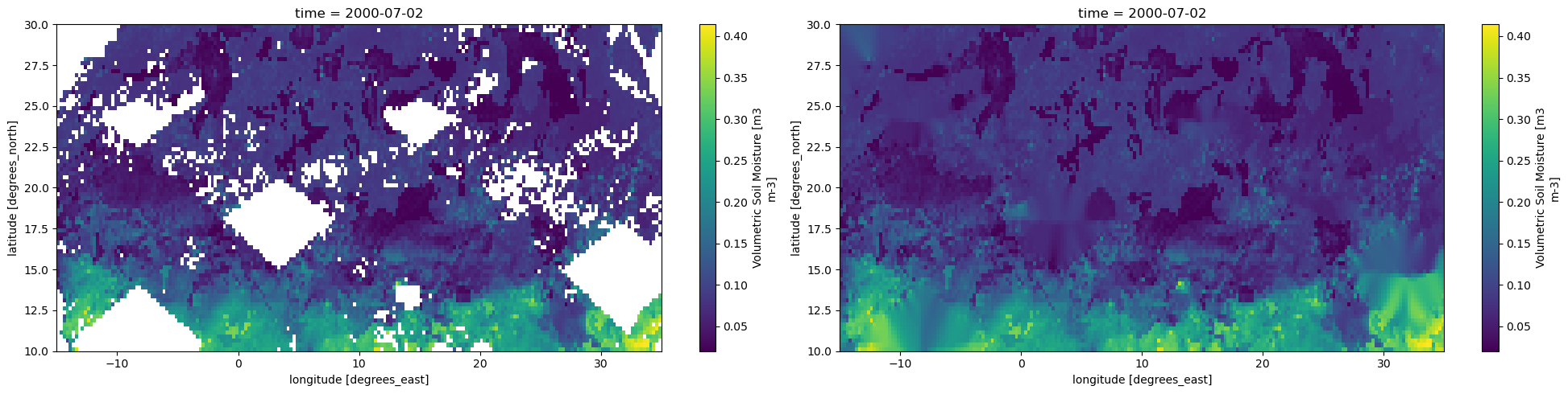
In this example, we utilize the low-pass gap-filling algorithm from `gridtools <https://github.com/esa-esdl/gridtools>`__ (DOI 10.5281/zenodo.15062839). This method effectively applies a 2D low-pass filter to the data. As a demonstration, we select a single time slice and apply gap filling in the spatial domain using the aforementioned algorithm.

sm_slice = ds.sm.sel(time='2000-07-01 12:00:00', method='nearest')
sm_slice

<xarray.DataArray 'sm' (lat: 720, lon: 1440)> Size: 4MB
dask.array<getitem, shape=(720, 1440), dtype=float32, chunksize=(720, 720), chunktype=numpy.ndarray>
Coordinates:
  * lat      (lat) float64 6kB 89.88 89.62 89.38 89.12 ... -89.38 -89.62 -89.88
  * lon      (lon) float64 12kB -179.9 -179.6 -179.4 ... 179.4 179.6 179.9
    time     datetime64[ns] 8B 2000-07-02
Attributes:
    _CoordinateAxes:      time lat lon
    ancillary_variables:  sm_uncertainty flag t0
    dtype:                float32
    long_name:            Volumetric Soil Moisture
    standard_name:        soil_moisture_content
    units:                m3 m-3
    valid_range:          [0.0, 1.0]

xarray.DataArray

'sm'

• lat: 720
• lon: 1440

• dask.array<chunksize=(720, 720), meta=np.ndarray>

  Array Chunk Bytes 3.96 MiB 1.98 MiB Shape (720, 1440) (720, 720) Dask graph 2 chunks in 3 graph layers Data type float32 numpy.ndarray

• Coordinates: (3)
  • lat
    (lat)
    float64
    89.88 89.62 89.38 ... -89.62 -89.88

    _CoordinateAxisType :

    Lat

    standard_name :

    latitude

    units :

    degrees_north

    valid_range :

    [-90.0, 90.0]

    array([ 89.875,  89.625,  89.375, ..., -89.375, -89.625, -89.875])

  • lon
    (lon)
    float64
    -179.9 -179.6 ... 179.6 179.9

    _CoordinateAxisType :

    Lon

    standard_name :

    longitude

    units :

    degrees_east

    valid_range :

    [-180.0, 180.0]

    array([-179.875, -179.625, -179.375, ...,  179.375,  179.625,  179.875])

  • time
    ()
    datetime64[ns]
    2000-07-02

    array('2000-07-02T00:00:00.000000000', dtype='datetime64[ns]')

• Indexes: (2)
  • lat
    PandasIndex

    PandasIndex(Index([ 89.875,  89.625,  89.375,  89.125,  88.875,  88.625,  88.375,  88.125,
            87.875,  87.625,
           ...
           -87.625, -87.875, -88.125, -88.375, -88.625, -88.875, -89.125, -89.375,
           -89.625, -89.875],
          dtype='float64', name='lat', length=720))

  • lon
    PandasIndex

    PandasIndex(Index([-179.875, -179.625, -179.375, -179.125, -178.875, -178.625, -178.375,
           -178.125, -177.875, -177.625,
           ...
            177.625,  177.875,  178.125,  178.375,  178.625,  178.875,  179.125,
            179.375,  179.625,  179.875],
          dtype='float64', name='lon', length=1440))

• Attributes: (7)

  _CoordinateAxes :

  time lat lon

  ancillary_variables :

  sm_uncertainty flag t0

  dtype :

  float32

  long_name :

  Volumetric Soil Moisture

  standard_name :

  soil_moisture_content

  units :

  m3 m-3

  valid_range :

  [0.0, 1.0]

ds_sub = ds.sel(time='2000-07-01 12:00:00', method='nearest')
ds_sub = ds_sub[["sm"]]
ds_sub

<xarray.Dataset> Size: 4MB
Dimensions:  (lat: 720, lon: 1440)
Coordinates:
  * lat      (lat) float64 6kB 89.88 89.62 89.38 89.12 ... -89.38 -89.62 -89.88
  * lon      (lon) float64 12kB -179.9 -179.6 -179.4 ... 179.4 179.6 179.9
    time     datetime64[ns] 8B 2000-07-02
Data variables:
    sm       (lat, lon) float32 4MB dask.array<chunksize=(720, 720), meta=np.ndarray>
Attributes: (12/44)
    Conventions:                  CF-1.9
    cdm_data_type:                Grid
    comment:                      This dataset was produced with funding of t...
    contact:                      cci_sm_contact@eodc.eu
    creator_email:                cci_sm_developer@eodc.eu
    creator_name:                 Department of Geodesy and Geoinformation, V...
    ...                           ...
    time_coverage_end_product:    20211231T235959Z
    time_coverage_resolution:     P1D
    time_coverage_start:          1978-11-01 00:00:00
    time_coverage_start_product:  19781101T000000Z
    title:                        ESA CCI Surface Soil Moisture COMBINED acti...
    tracking_id:                  ad35798e-58e0-488f-b5b9-593874a47700

xarray.Dataset

• Dimensions:
  • lat: 720
  • lon: 1440
• Coordinates: (3)
  • lat
    (lat)
    float64
    89.88 89.62 89.38 ... -89.62 -89.88

    _CoordinateAxisType :

    Lat

    standard_name :

    latitude

    units :

    degrees_north

    valid_range :

    [-90.0, 90.0]

    array([ 89.875,  89.625,  89.375, ..., -89.375, -89.625, -89.875])

  • lon
    (lon)
    float64
    -179.9 -179.6 ... 179.6 179.9

    _CoordinateAxisType :

    Lon

    standard_name :

    longitude

    units :

    degrees_east

    valid_range :

    [-180.0, 180.0]

    array([-179.875, -179.625, -179.375, ...,  179.375,  179.625,  179.875])

  • time
    ()
    datetime64[ns]
    2000-07-02

    array('2000-07-02T00:00:00.000000000', dtype='datetime64[ns]')

• Data variables: (1)
  • sm
    (lat, lon)
    float32
    dask.array<chunksize=(720, 720), meta=np.ndarray>

    _CoordinateAxes :

    time lat lon

    ancillary_variables :

    sm_uncertainty flag t0

    dtype :

    float32

    long_name :

    Volumetric Soil Moisture

    standard_name :

    soil_moisture_content

    units :

    m3 m-3

    valid_range :

    [0.0, 1.0]

    Array Chunk Bytes 3.96 MiB 1.98 MiB Shape (720, 1440) (720, 720) Dask graph 2 chunks in 3 graph layers Data type float32 numpy.ndarray

• Indexes: (2)
  • lat
    PandasIndex

    PandasIndex(Index([ 89.875,  89.625,  89.375,  89.125,  88.875,  88.625,  88.375,  88.125,
            87.875,  87.625,
           ...
           -87.625, -87.875, -88.125, -88.375, -88.625, -88.875, -89.125, -89.375,
           -89.625, -89.875],
          dtype='float64', name='lat', length=720))

  • lon
    PandasIndex

    PandasIndex(Index([-179.875, -179.625, -179.375, -179.125, -178.875, -178.625, -178.375,
           -178.125, -177.875, -177.625,
           ...
            177.625,  177.875,  178.125,  178.375,  178.625,  178.875,  179.125,
            179.375,  179.625,  179.875],
          dtype='float64', name='lon', length=1440))

• Attributes: (44)

  Conventions :

  CF-1.9

  cdm_data_type :

  Grid

  comment :

  This dataset was produced with funding of the ESA CCI+ Soil Moisture project; ESRIN Contract No: 4000126684/19/I-NB

  contact :

  cci_sm_contact@eodc.eu

  creator_email :

  cci_sm_developer@eodc.eu

  creator_name :

  Department of Geodesy and Geoinformation, Vienna University of Technology

  creator_url :

  https://climers.geo.tuwien.ac.at/

  date_created :

  File created: 2022-04-06 12:31:39.526359

  geospatial_lat_max :

  90.0

  geospatial_lat_min :

  -90.0

  geospatial_lat_resolution :

  0.25 degree

  geospatial_lat_units :

  degrees_north

  geospatial_lon_max :

  180.0

  geospatial_lon_min :

  -180.0

  geospatial_lon_resolution :

  0.25 degree

  geospatial_lon_units :

  degrees_east

  geospatial_vertical_max :

  0.0

  geospatial_vertical_min :

  0.0

  history :

  2022-04-06 12:29:35 - product produced 2023-08-09 17:33:51 - converted by nc2zarr, version 1.1.2.dev0

  id :

  ESACCI-SOILMOISTURE-L3S-SSMV-COMBINED-20211231000000-fv07.1.nc

  institution :

  TU Wien (AUT); VanderSat B.V. (NL)

  key_variables :

  sm

  keywords :

  soil moisture, soil water content, microwave remote sensing, active, passive, combined, climate data record

  keywords_vocabulary :

  NASA Global Change Master Directory (GCMD) Science Keywords

  license :

  Data use is free and open for all registered users.

  naming_authority :

  TU Wien

  platform :

  Nimbus 7, DMSP, TRMM, AQUA, Coriolis, GCOM-W1, MIRAS, SMAP, GPM, FengYun-3B, FengYun-3C, FengYun-3D; ERS-1, ERS-2, METOP-A, METOP-B

  processing_level :

  Quality-controlled, super-collocated (L3S) Satellite Soil Moisture (SM) data from multiple sensors

  product_version :

  v07.1

  project :

  Climate Change Initiative - European Space Agency

  references :

  http://www.esa-soilmoisture-cci.org; Dorigo, W.A., Wagner, W., Albergel, C., Albrecht, F., Balsamo, G., Brocca, L., Chung, D., Ertl, M., Forkel, M., Gruber, A., Haas, E., Hamer, D. P. Hirschi, M., Ikonen, J., De Jeu, R. Kidd, R. Lahoz, W., Liu, Y.Y., Miralles, D., Lecomte, P. (2017) ESA CCI Soil Moisture for improved Earth system understanding: State-of-the art and future directions. In Remote Sensing of Environment, 2017, ISSN 0034-4257, https://doi.org/10.1016/j.rse.2017.07.001; Gruber, A., Scanlon, T., van der Schalie, R., Wagner, W., Dorigo, W. (2019) Evolution of the ESA CCI Soil Moisture Climate Data Records and their underlying merging methodology. Earth System Science Data 11, 717-739, https://doi.org/10.5194/essd-11-717-2019; Gruber, A., Dorigo, W. A., Crow, W., Wagner W. (2017). Triple Collocation-Based Merging of Satellite Soil Moisture Retrievals. IEEE Transactions on Geoscience and Remote Sensing. PP. 1-13. https://doi.org/10.1109/TGRS.2017.2734070

  sensor :

  SMMR, SSM/I, TMI, AMSR-E, WindSat, AMSR2, SMOS, SMAP_radiometer, GMI, VIRR-3B, VIRR-3C, VIRR-3D; AMI-WS, ASCAT-A, ASCAT-B, ASCAT-C

  source :

  WARP 5.5R1.1/AMI-WS/ERS12 Level 2 Soil Moisture; WARP 5.4R1.0/AMI-WS/ERS2 Level 2 Soil Moisture; H115: Metop ASCAT Surface Soil Moisture Climate Data Record v5 12.5 km sampling, DOI: 10.15770/EUM_SAF_H_0006; H116: Metop ASCAT Surface Soil Moisture Climate Data Record v5 Extension 12.5 km sampling; H115: Metop ASCAT Surface Soil Moisture Climate Data Record v5 12.5 km sampling, DOI: 10.15770/EUM_SAF_H_0006; H116: Metop ASCAT Surface Soil Moisture Climate Data Record v5 Extension 12.5 km sampling; H115: Metop ASCAT Surface Soil Moisture Climate Data Record v5 12.5 km sampling, DOI: 10.15770/EUM_SAF_H_0006; H116: Metop ASCAT Surface Soil Moisture Climate Data Record v5 Extension 12.5 km sampling;; LPRMv7/SMMR/Nimbus 7 L3 Surface Soil Moisture, Ancillary Params, and quality flags; LPRMv7/SSMI/F08, F11, F13 DMSP L3 Surface Soil Moisture, Ancillary Params, and quality flags; LPRMv7/TMI/TRMM L2 Surface Soil Moisture, Ancillary Params, and QC; LPRMv7/AMSR-E/Aqua L2B Surface Soil Moisture, Ancillary Params, and QC; LPRMv7/WINDSAT/CORIOLIS L2 Surface Soil Moisture, Ancillary Params, and QC; LPRMv7/AMSR2/GCOM-W1 L3 Surface Soil Moisture, Ancillary Params; LPRMv7/SMOS/MIRAS L3 Surface Soil Moisture, CATDS Level 3 Brightness Temperatures (L3TB) version 300 RE03 & RE04; LPRMv7/SMAP_radiometer/SMAP L2 Surface Soil Moisture, Ancillary Params, and QC; LPRMv7/GMI/GPM L3 Surface Soil Moisture, Ancillary Params, and quality flags; LPRMv7/VIRR/FengYun-3B L3 Surface Soil Moisture, Ancillary Params, and quality flags; LPRMv7/VIRR/FengYun-3C L3 Surface Soil Moisture, Ancillary Params, and quality flags; LPRMv7/VIRR/FengYun-3D L3 Surface Soil Moisture, Ancillary Params, and quality flags;;

  spatial_resolution :

  25km

  standard_name_vocabulary :

  CF Standard Name Table v77

  summary :

  This dataset was produced with funding of the ESA CCI+ Soil Moisture project; ESRIN Contract No: 4000126684/19/I-NB

  time_coverage_duration :

  P43Y

  time_coverage_end :

  2021-12-31 00:00:00

  time_coverage_end_product :

  20211231T235959Z

  time_coverage_resolution :

  P1D

  time_coverage_start :

  1978-11-01 00:00:00

  time_coverage_start_product :

  19781101T000000Z

  title :

  ESA CCI Surface Soil Moisture COMBINED active+passive Product

  tracking_id :

  ad35798e-58e0-488f-b5b9-593874a47700

Next, we apply the toolbox’s gap-filling operation, which is highly efficient as it leverages Numba for parallel computation.

gapfill_op = get_op('gapfill')

ds_filled = gapfill_op(ds_sub)
ds_filled.sm

<xarray.DataArray 'sm' (lat: 720, lon: 1440)> Size: 4MB
dask.array<fillgaps_lowpass_2d, shape=(720, 1440), dtype=float32, chunksize=(720, 720), chunktype=numpy.ndarray>
Coordinates:
  * lat      (lat) float64 6kB 89.88 89.62 89.38 89.12 ... -89.38 -89.62 -89.88
  * lon      (lon) float64 12kB -179.9 -179.6 -179.4 ... 179.4 179.6 179.9
    time     datetime64[ns] 8B 2000-07-02
Attributes:
    _CoordinateAxes:      time lat lon
    ancillary_variables:  sm_uncertainty flag t0
    dtype:                float32
    long_name:            Volumetric Soil Moisture
    standard_name:        soil_moisture_content
    units:                m3 m-3
    valid_range:          [0.0, 1.0]

xarray.DataArray

'sm'

• lat: 720
• lon: 1440

• dask.array<chunksize=(720, 720), meta=np.ndarray>

  Array Chunk Bytes 3.96 MiB 1.98 MiB Shape (720, 1440) (720, 720) Dask graph 2 chunks in 4 graph layers Data type float32 numpy.ndarray

• Coordinates: (3)
  • lat
    (lat)
    float64
    89.88 89.62 89.38 ... -89.62 -89.88

    _CoordinateAxisType :

    Lat

    standard_name :

    latitude

    units :

    degrees_north

    valid_range :

    [-90.0, 90.0]

    array([ 89.875,  89.625,  89.375, ..., -89.375, -89.625, -89.875])

  • lon
    (lon)
    float64
    -179.9 -179.6 ... 179.6 179.9

    _CoordinateAxisType :

    Lon

    standard_name :

    longitude

    units :

    degrees_east

    valid_range :

    [-180.0, 180.0]

    array([-179.875, -179.625, -179.375, ...,  179.375,  179.625,  179.875])

  • time
    ()
    datetime64[ns]
    2000-07-02

    array('2000-07-02T00:00:00.000000000', dtype='datetime64[ns]')

• Indexes: (2)
  • lat
    PandasIndex

    PandasIndex(Index([ 89.875,  89.625,  89.375,  89.125,  88.875,  88.625,  88.375,  88.125,
            87.875,  87.625,
           ...
           -87.625, -87.875, -88.125, -88.375, -88.625, -88.875, -89.125, -89.375,
           -89.625, -89.875],
          dtype='float64', name='lat', length=720))

  • lon
    PandasIndex

    PandasIndex(Index([-179.875, -179.625, -179.375, -179.125, -178.875, -178.625, -178.375,
           -178.125, -177.875, -177.625,
           ...
            177.625,  177.875,  178.125,  178.375,  178.625,  178.875,  179.125,
            179.375,  179.625,  179.875],
          dtype='float64', name='lon', length=1440))

• Attributes: (7)

  _CoordinateAxes :

  time lat lon

  ancillary_variables :

  sm_uncertainty flag t0

  dtype :

  float32

  long_name :

  Volumetric Soil Moisture

  standard_name :

  soil_moisture_content

  units :

  m3 m-3

  valid_range :

  [0.0, 1.0]

Finally, we plot the results for North Africa as an example to illustrate the gap-filling process.

fig, ax = plt.subplots(1, 2, figsize=(20, 5))
extent = dict(lat=slice(30, 10), lon=slice(-15, 35))
ds_sub.sm.sel(**extent).plot(ax=ax[0])
ds_filled.sm.sel(**extent).plot(ax=ax[1])

<matplotlib.collections.QuadMesh at 0x785408428f50>