4.2.2.4. Filter Operations

In this section, we will demonstrate three filter operations on CCI ECV datasets:

1. Filtering a dataset based on a specific flag value.

2. Filtering, exploring, and propagating uncertainties that accompany the dataset.

3. Filtering based on any data feature.

All of these filter operations are performed using the `xarray.Dataset.where <https://docs.xarray.dev/en/stable/generated/xarray.Dataset.where.html>`__ method, which is fully compatible with Dask. This approach allows for on-demand filtering, performed chunk-by-chunk for efficiency.

---

4.2.2.4.1. 1. Filtering a datset for a given flag value

We will show this filtering operation on a soil moisture dataset, which comes with a quality flag for its observational data.

import matplotlib.pyplot as plt
from xcube.core.store import new_data_store

We can access the soil moisture dataset through the Zarr data store, as shown below:

store = new_data_store('esa-cci-zarr')

ds = store.open_data("ESACCI-SOILMOISTURE-L3S-SSMV-COMBINED-1978-2021-fv07.1.zarr")
ds

<xarray.Dataset> Size: 654GB
Dimensions:         (time: 15767, lat: 720, lon: 1440)
Coordinates:
  * lat             (lat) float64 6kB 89.88 89.62 89.38 ... -89.38 -89.62 -89.88
  * lon             (lon) float64 12kB -179.9 -179.6 -179.4 ... 179.6 179.9
  * time            (time) datetime64[ns] 126kB 1978-11-01 ... 2021-12-31
Data variables:
    dnflag          (time, lat, lon) float32 65GB dask.array<chunksize=(16, 720, 720), meta=np.ndarray>
    flag            (time, lat, lon) float32 65GB dask.array<chunksize=(16, 720, 720), meta=np.ndarray>
    freqbandID      (time, lat, lon) float32 65GB dask.array<chunksize=(16, 720, 720), meta=np.ndarray>
    mode            (time, lat, lon) float32 65GB dask.array<chunksize=(16, 720, 720), meta=np.ndarray>
    sensor          (time, lat, lon) float64 131GB dask.array<chunksize=(16, 720, 720), meta=np.ndarray>
    sm              (time, lat, lon) float32 65GB dask.array<chunksize=(16, 720, 720), meta=np.ndarray>
    sm_uncertainty  (time, lat, lon) float32 65GB dask.array<chunksize=(16, 720, 720), meta=np.ndarray>
    t0              (time, lat, lon) float64 131GB dask.array<chunksize=(16, 720, 720), meta=np.ndarray>
Attributes: (12/44)
    Conventions:                  CF-1.9
    cdm_data_type:                Grid
    comment:                      This dataset was produced with funding of t...
    contact:                      cci_sm_contact@eodc.eu
    creator_email:                cci_sm_developer@eodc.eu
    creator_name:                 Department of Geodesy and Geoinformation, V...
    ...                           ...
    time_coverage_end_product:    20211231T235959Z
    time_coverage_resolution:     P1D
    time_coverage_start:          1978-11-01 00:00:00
    time_coverage_start_product:  19781101T000000Z
    title:                        ESA CCI Surface Soil Moisture COMBINED acti...
    tracking_id:                  ad35798e-58e0-488f-b5b9-593874a47700

xarray.Dataset

• Dimensions:
  • time: 15767
  • lat: 720
  • lon: 1440
• Coordinates: (3)
  • lat
    (lat)
    float64
    89.88 89.62 89.38 ... -89.62 -89.88

    _CoordinateAxisType :

    Lat

    standard_name :

    latitude

    units :

    degrees_north

    valid_range :

    [-90.0, 90.0]

    array([ 89.875,  89.625,  89.375, ..., -89.375, -89.625, -89.875])

  • lon
    (lon)
    float64
    -179.9 -179.6 ... 179.6 179.9

    _CoordinateAxisType :

    Lon

    standard_name :

    longitude

    units :

    degrees_east

    valid_range :

    [-180.0, 180.0]

    array([-179.875, -179.625, -179.375, ...,  179.375,  179.625,  179.875])

  • time
    (time)
    datetime64[ns]
    1978-11-01 ... 2021-12-31

    array(['1978-11-01T00:00:00.000000000', '1978-11-02T00:00:00.000000000',
           '1978-11-03T00:00:00.000000000', ..., '2021-12-29T00:00:00.000000000',
           '2021-12-30T00:00:00.000000000', '2021-12-31T00:00:00.000000000'],
          dtype='datetime64[ns]')

• Data variables: (8)
  • dnflag
    (time, lat, lon)
    float32
    dask.array<chunksize=(16, 720, 720), meta=np.ndarray>

    _CoordinateAxes :

    time lat lon

    bit_meanings :

    ['NaN', 'day', 'night']

    bits :

    ['0b0', '0b1', '0b10']

    dtype :

    int8

    flag_meanings :

    ['NaN', 'day', 'night', 'day_night_combination']

    flag_values :

    [0, 1, 2, 3]

    long_name :

    Day / Night Flag

    valid_range :

    [0, 3]

    Array Chunk Bytes 60.90 GiB 31.64 MiB Shape (15767, 720, 1440) (16, 720, 720) Dask graph 1972 chunks in 2 graph layers Data type float32 numpy.ndarray

  • flag
    (time, lat, lon)
    float32
    dask.array<chunksize=(16, 720, 720), meta=np.ndarray>

    _CoordinateAxes :

    time lat lon

    bit_meanings :

    ['no_data_inconsistency_detected', 'snow_coverage_or_temperature_below_zero', 'dense_vegetation', 'others_no_convergence_in_the_model_thus_no_valid_sm_estimates', 'soil_moisture_value_exceeds_physical_boundary', 'weight_of_measurement_below_threshold', 'all_datasets_deemed_unreliable', 'barren_ground_advisory_flag', 'NaN']

    bits :

    ['0b0', '0b1', '0b10', '0b100', '0b1000', '0b10000', '0b100000', '0b1000000', '0b10000000']

    dtype :

    int16

    flag_meanings :

    ['no_data_inconsistency_detected', 'snow_coverage_or_temperature_below_zero', 'dense_vegetation', 'combination_of_flag_values_1_and_2', 'soil_moisture_value_exceeds_physical_boundary', 'combination_of_flag_values_1_and_8', 'combination_of_flag_values_2_and_8', 'barren_ground_advisory_flag', 'combination_of_flag_values_1_and_64', 'combination_of_flag_values_2_and_64', 'combination_of_flag_values_1_and_2_and_64', 'combination_of_flag_values_8_and_64', 'combination_of_flag_values_1_and_8_and_64', 'combination_of_flag_values_2_and_8_and_64', 'combination_of_flag_values_1_and_2_and_4_and_8_and_16_and_32_and_64']

    flag_values :

    [0, 1, 2, 3, 8, 9, 10, 64, 65, 66, 67, 72, 73, 74, 127]

    long_name :

    Flag

    standard_name :

    soil_moisture_content status_flag

    valid_range :

    [0, 255]

    Array Chunk Bytes 60.90 GiB 31.64 MiB Shape (15767, 720, 1440) (16, 720, 720) Dask graph 1972 chunks in 2 graph layers Data type float32 numpy.ndarray

  • freqbandID
    (time, lat, lon)
    float32
    dask.array<chunksize=(16, 720, 720), meta=np.ndarray>

    _CoordinateAxes :

    time lat lon

    bit_meanings :

    ['NaN', 'L14', 'C53', 'C66', 'C68', 'C69', 'C73', 'X107', 'K194', 'MODEL']

    bits :

    ['0b0', '0b1', '0b10', '0b100', '0b1000', '0b10000', '0b100000', '0b1000000', '0b10000000', '0b100000000']

    dtype :

    int16

    flag_meanings :

    ['NaN', 'C66', 'X107', 'C66+X107']

    flag_values :

    [0, 4, 64, 68]

    long_name :

    Frequency Band Identification

    valid_range :

    [0, 511]

    Array Chunk Bytes 60.90 GiB 31.64 MiB Shape (15767, 720, 1440) (16, 720, 720) Dask graph 1972 chunks in 2 graph layers Data type float32 numpy.ndarray

  • mode
    (time, lat, lon)
    float32
    dask.array<chunksize=(16, 720, 720), meta=np.ndarray>

    _CoordinateAxes :

    time lat lon

    bit_meanings :

    ['NaN', 'ascending', 'descending']

    bits :

    ['0b0', '0b1', '0b10']

    dtype :

    int8

    flag_meanings :

    ['NaN', 'ascending', 'descending', 'ascending_descending_combination']

    flag_values :

    [0, 1, 2, 3]

    long_name :

    Satellite Mode

    valid_range :

    [0, 3]

    Array Chunk Bytes 60.90 GiB 31.64 MiB Shape (15767, 720, 1440) (16, 720, 720) Dask graph 1972 chunks in 2 graph layers Data type float32 numpy.ndarray

  • sensor
    (time, lat, lon)
    float64
    dask.array<chunksize=(16, 720, 720), meta=np.ndarray>

    _CoordinateAxes :

    time lat lon

    bit_meanings :

    ['NaN', 'SMMR', 'SSMI', 'TMI', 'AMSRE', 'WindSat', 'AMSR2', 'SMOS', 'AMIWS', 'ASCATA', 'ASCATB', 'SMAP', 'MODEL', 'GPM', 'FY3B', 'FY3D', 'ASCATC', 'FY3C']

    bits :

    ['0b0', '0b1', '0b10', '0b100', '0b1000', '0b10000', '0b100000', '0b1000000', '0b10000000', '0b100000000', '0b1000000000', '0b10000000000', '0b100000000000', '0b1000000000000', '0b10000000000000', '0b100000000000000', '0b1000000000000000', '0b10000000000000000']

    dtype :

    int32

    flag_meanings :

    ['NaN', 'SMMR']

    flag_values :

    [0, 1]

    long_name :

    Sensor

    valid_range :

    [0, 131071]

    Array Chunk Bytes 121.80 GiB 63.28 MiB Shape (15767, 720, 1440) (16, 720, 720) Dask graph 1972 chunks in 2 graph layers Data type float64 numpy.ndarray

  • sm
    (time, lat, lon)
    float32
    dask.array<chunksize=(16, 720, 720), meta=np.ndarray>

    _CoordinateAxes :

    time lat lon

    ancillary_variables :

    sm_uncertainty flag t0

    dtype :

    float32

    long_name :

    Volumetric Soil Moisture

    standard_name :

    soil_moisture_content

    units :

    m3 m-3

    valid_range :

    [0.0, 1.0]

    Array Chunk Bytes 60.90 GiB 31.64 MiB Shape (15767, 720, 1440) (16, 720, 720) Dask graph 1972 chunks in 2 graph layers Data type float32 numpy.ndarray

  • sm_uncertainty
    (time, lat, lon)
    float32
    dask.array<chunksize=(16, 720, 720), meta=np.ndarray>

    _CoordinateAxes :

    time lat lon

    dtype :

    float32

    long_name :

    Volumetric Soil Moisture Uncertainty

    standard_name :

    soil_moisture_content standard_error

    units :

    m3 m-3

    valid_range :

    [0.0, 1.0]

    Array Chunk Bytes 60.90 GiB 31.64 MiB Shape (15767, 720, 1440) (16, 720, 720) Dask graph 1972 chunks in 2 graph layers Data type float32 numpy.ndarray

  • t0
    (time, lat, lon)
    float64
    dask.array<chunksize=(16, 720, 720), meta=np.ndarray>

    _CoordinateAxes :

    time lat lon

    dtype :

    float64

    long_name :

    Observation Timestamp

    units :

    days after 1970-01-01 00:00:00 UTC

    valid_range :

    [3225.0, 3227.0]

    Array Chunk Bytes 121.80 GiB 63.28 MiB Shape (15767, 720, 1440) (16, 720, 720) Dask graph 1972 chunks in 2 graph layers Data type float64 numpy.ndarray

• Indexes: (3)
  • lat
    PandasIndex

    PandasIndex(Index([ 89.875,  89.625,  89.375,  89.125,  88.875,  88.625,  88.375,  88.125,
            87.875,  87.625,
           ...
           -87.625, -87.875, -88.125, -88.375, -88.625, -88.875, -89.125, -89.375,
           -89.625, -89.875],
          dtype='float64', name='lat', length=720))

  • lon
    PandasIndex

    PandasIndex(Index([-179.875, -179.625, -179.375, -179.125, -178.875, -178.625, -178.375,
           -178.125, -177.875, -177.625,
           ...
            177.625,  177.875,  178.125,  178.375,  178.625,  178.875,  179.125,
            179.375,  179.625,  179.875],
          dtype='float64', name='lon', length=1440))

  • time
    PandasIndex

    PandasIndex(DatetimeIndex(['1978-11-01', '1978-11-02', '1978-11-03', '1978-11-04',
                   '1978-11-05', '1978-11-06', '1978-11-07', '1978-11-08',
                   '1978-11-09', '1978-11-10',
                   ...
                   '2021-12-22', '2021-12-23', '2021-12-24', '2021-12-25',
                   '2021-12-26', '2021-12-27', '2021-12-28', '2021-12-29',
                   '2021-12-30', '2021-12-31'],
                  dtype='datetime64[ns]', name='time', length=15767, freq=None))

• Attributes: (44)

  Conventions :

  CF-1.9

  cdm_data_type :

  Grid

  comment :

  This dataset was produced with funding of the ESA CCI+ Soil Moisture project; ESRIN Contract No: 4000126684/19/I-NB

  contact :

  cci_sm_contact@eodc.eu

  creator_email :

  cci_sm_developer@eodc.eu

  creator_name :

  Department of Geodesy and Geoinformation, Vienna University of Technology

  creator_url :

  https://climers.geo.tuwien.ac.at/

  date_created :

  File created: 2022-04-06 12:31:39.526359

  geospatial_lat_max :

  90.0

  geospatial_lat_min :

  -90.0

  geospatial_lat_resolution :

  0.25 degree

  geospatial_lat_units :

  degrees_north

  geospatial_lon_max :

  180.0

  geospatial_lon_min :

  -180.0

  geospatial_lon_resolution :

  0.25 degree

  geospatial_lon_units :

  degrees_east

  geospatial_vertical_max :

  0.0

  geospatial_vertical_min :

  0.0

  history :

  2022-04-06 12:29:35 - product produced 2023-08-09 17:33:51 - converted by nc2zarr, version 1.1.2.dev0

  id :

  ESACCI-SOILMOISTURE-L3S-SSMV-COMBINED-20211231000000-fv07.1.nc

  institution :

  TU Wien (AUT); VanderSat B.V. (NL)

  key_variables :

  sm

  keywords :

  soil moisture, soil water content, microwave remote sensing, active, passive, combined, climate data record

  keywords_vocabulary :

  NASA Global Change Master Directory (GCMD) Science Keywords

  license :

  Data use is free and open for all registered users.

  naming_authority :

  TU Wien

  platform :

  Nimbus 7, DMSP, TRMM, AQUA, Coriolis, GCOM-W1, MIRAS, SMAP, GPM, FengYun-3B, FengYun-3C, FengYun-3D; ERS-1, ERS-2, METOP-A, METOP-B

  processing_level :

  Quality-controlled, super-collocated (L3S) Satellite Soil Moisture (SM) data from multiple sensors

  product_version :

  v07.1

  project :

  Climate Change Initiative - European Space Agency

  references :

  http://www.esa-soilmoisture-cci.org; Dorigo, W.A., Wagner, W., Albergel, C., Albrecht, F., Balsamo, G., Brocca, L., Chung, D., Ertl, M., Forkel, M., Gruber, A., Haas, E., Hamer, D. P. Hirschi, M., Ikonen, J., De Jeu, R. Kidd, R. Lahoz, W., Liu, Y.Y., Miralles, D., Lecomte, P. (2017) ESA CCI Soil Moisture for improved Earth system understanding: State-of-the art and future directions. In Remote Sensing of Environment, 2017, ISSN 0034-4257, https://doi.org/10.1016/j.rse.2017.07.001; Gruber, A., Scanlon, T., van der Schalie, R., Wagner, W., Dorigo, W. (2019) Evolution of the ESA CCI Soil Moisture Climate Data Records and their underlying merging methodology. Earth System Science Data 11, 717-739, https://doi.org/10.5194/essd-11-717-2019; Gruber, A., Dorigo, W. A., Crow, W., Wagner W. (2017). Triple Collocation-Based Merging of Satellite Soil Moisture Retrievals. IEEE Transactions on Geoscience and Remote Sensing. PP. 1-13. https://doi.org/10.1109/TGRS.2017.2734070

  sensor :

  SMMR, SSM/I, TMI, AMSR-E, WindSat, AMSR2, SMOS, SMAP_radiometer, GMI, VIRR-3B, VIRR-3C, VIRR-3D; AMI-WS, ASCAT-A, ASCAT-B, ASCAT-C

  source :

  WARP 5.5R1.1/AMI-WS/ERS12 Level 2 Soil Moisture; WARP 5.4R1.0/AMI-WS/ERS2 Level 2 Soil Moisture; H115: Metop ASCAT Surface Soil Moisture Climate Data Record v5 12.5 km sampling, DOI: 10.15770/EUM_SAF_H_0006; H116: Metop ASCAT Surface Soil Moisture Climate Data Record v5 Extension 12.5 km sampling; H115: Metop ASCAT Surface Soil Moisture Climate Data Record v5 12.5 km sampling, DOI: 10.15770/EUM_SAF_H_0006; H116: Metop ASCAT Surface Soil Moisture Climate Data Record v5 Extension 12.5 km sampling; H115: Metop ASCAT Surface Soil Moisture Climate Data Record v5 12.5 km sampling, DOI: 10.15770/EUM_SAF_H_0006; H116: Metop ASCAT Surface Soil Moisture Climate Data Record v5 Extension 12.5 km sampling;; LPRMv7/SMMR/Nimbus 7 L3 Surface Soil Moisture, Ancillary Params, and quality flags; LPRMv7/SSMI/F08, F11, F13 DMSP L3 Surface Soil Moisture, Ancillary Params, and quality flags; LPRMv7/TMI/TRMM L2 Surface Soil Moisture, Ancillary Params, and QC; LPRMv7/AMSR-E/Aqua L2B Surface Soil Moisture, Ancillary Params, and QC; LPRMv7/WINDSAT/CORIOLIS L2 Surface Soil Moisture, Ancillary Params, and QC; LPRMv7/AMSR2/GCOM-W1 L3 Surface Soil Moisture, Ancillary Params; LPRMv7/SMOS/MIRAS L3 Surface Soil Moisture, CATDS Level 3 Brightness Temperatures (L3TB) version 300 RE03 & RE04; LPRMv7/SMAP_radiometer/SMAP L2 Surface Soil Moisture, Ancillary Params, and QC; LPRMv7/GMI/GPM L3 Surface Soil Moisture, Ancillary Params, and quality flags; LPRMv7/VIRR/FengYun-3B L3 Surface Soil Moisture, Ancillary Params, and quality flags; LPRMv7/VIRR/FengYun-3C L3 Surface Soil Moisture, Ancillary Params, and quality flags; LPRMv7/VIRR/FengYun-3D L3 Surface Soil Moisture, Ancillary Params, and quality flags;;

  spatial_resolution :

  25km

  standard_name_vocabulary :

  CF Standard Name Table v77

  summary :

  This dataset was produced with funding of the ESA CCI+ Soil Moisture project; ESRIN Contract No: 4000126684/19/I-NB

  time_coverage_duration :

  P43Y

  time_coverage_end :

  2021-12-31 00:00:00

  time_coverage_end_product :

  20211231T235959Z

  time_coverage_resolution :

  P1D

  time_coverage_start :

  1978-11-01 00:00:00

  time_coverage_start_product :

  19781101T000000Z

  title :

  ESA CCI Surface Soil Moisture COMBINED active+passive Product

  tracking_id :

  ad35798e-58e0-488f-b5b9-593874a47700

We can filter the soil moisture data using the "no_data_inconsistency_detected" flag, which corresponds to a flag value of 0 in the flag data variable. This value can be verified by checking the attributes of the flag variable.

filtered_ds = ds.where(ds["flag"] != 0)
filtered_ds

<xarray.Dataset> Size: 654GB
Dimensions:         (time: 15767, lat: 720, lon: 1440)
Coordinates:
  * lat             (lat) float64 6kB 89.88 89.62 89.38 ... -89.38 -89.62 -89.88
  * lon             (lon) float64 12kB -179.9 -179.6 -179.4 ... 179.6 179.9
  * time            (time) datetime64[ns] 126kB 1978-11-01 ... 2021-12-31
Data variables:
    dnflag          (time, lat, lon) float32 65GB dask.array<chunksize=(16, 720, 720), meta=np.ndarray>
    flag            (time, lat, lon) float32 65GB dask.array<chunksize=(16, 720, 720), meta=np.ndarray>
    freqbandID      (time, lat, lon) float32 65GB dask.array<chunksize=(16, 720, 720), meta=np.ndarray>
    mode            (time, lat, lon) float32 65GB dask.array<chunksize=(16, 720, 720), meta=np.ndarray>
    sensor          (time, lat, lon) float64 131GB dask.array<chunksize=(16, 720, 720), meta=np.ndarray>
    sm              (time, lat, lon) float32 65GB dask.array<chunksize=(16, 720, 720), meta=np.ndarray>
    sm_uncertainty  (time, lat, lon) float32 65GB dask.array<chunksize=(16, 720, 720), meta=np.ndarray>
    t0              (time, lat, lon) float64 131GB dask.array<chunksize=(16, 720, 720), meta=np.ndarray>
Attributes: (12/44)
    Conventions:                  CF-1.9
    cdm_data_type:                Grid
    comment:                      This dataset was produced with funding of t...
    contact:                      cci_sm_contact@eodc.eu
    creator_email:                cci_sm_developer@eodc.eu
    creator_name:                 Department of Geodesy and Geoinformation, V...
    ...                           ...
    time_coverage_end_product:    20211231T235959Z
    time_coverage_resolution:     P1D
    time_coverage_start:          1978-11-01 00:00:00
    time_coverage_start_product:  19781101T000000Z
    title:                        ESA CCI Surface Soil Moisture COMBINED acti...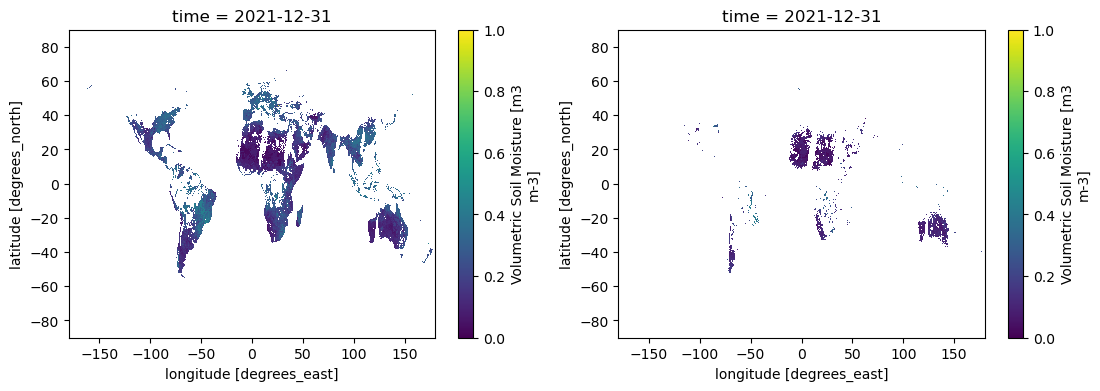
    tracking_id:                  ad35798e-58e0-488f-b5b9-593874a47700

xarray.Dataset

• Dimensions:
  • time: 15767
  • lat: 720
  • lon: 1440
• Coordinates: (3)
  • lat
    (lat)
    float64
    89.88 89.62 89.38 ... -89.62 -89.88

    _CoordinateAxisType :

    Lat

    standard_name :

    latitude

    units :

    degrees_north

    valid_range :

    [-90.0, 90.0]

    array([ 89.875,  89.625,  89.375, ..., -89.375, -89.625, -89.875])

  • lon
    (lon)
    float64
    -179.9 -179.6 ... 179.6 179.9

    _CoordinateAxisType :

    Lon

    standard_name :

    longitude

    units :

    degrees_east

    valid_range :

    [-180.0, 180.0]

    array([-179.875, -179.625, -179.375, ...,  179.375,  179.625,  179.875])

  • time
    (time)
    datetime64[ns]
    1978-11-01 ... 2021-12-31

    array(['1978-11-01T00:00:00.000000000', '1978-11-02T00:00:00.000000000',
           '1978-11-03T00:00:00.000000000', ..., '2021-12-29T00:00:00.000000000',
           '2021-12-30T00:00:00.000000000', '2021-12-31T00:00:00.000000000'],
          dtype='datetime64[ns]')

• Data variables: (8)
  • dnflag
    (time, lat, lon)
    float32
    dask.array<chunksize=(16, 720, 720), meta=np.ndarray>

    _CoordinateAxes :

    time lat lon

    bit_meanings :

    ['NaN', 'day', 'night']

    bits :

    ['0b0', '0b1', '0b10']

    dtype :

    int8

    flag_meanings :

    ['NaN', 'day', 'night', 'day_night_combination']

    flag_values :

    [0, 1, 2, 3]

    long_name :

    Day / Night Flag

    valid_range :

    [0, 3]

    Array Chunk Bytes 60.90 GiB 31.64 MiB Shape (15767, 720, 1440) (16, 720, 720) Dask graph 1972 chunks in 6 graph layers Data type float32 numpy.ndarray

  • flag
    (time, lat, lon)
    float32
    dask.array<chunksize=(16, 720, 720), meta=np.ndarray>

    _CoordinateAxes :

    time lat lon

    bit_meanings :

    ['no_data_inconsistency_detected', 'snow_coverage_or_temperature_below_zero', 'dense_vegetation', 'others_no_convergence_in_the_model_thus_no_valid_sm_estimates', 'soil_moisture_value_exceeds_physical_boundary', 'weight_of_measurement_below_threshold', 'all_datasets_deemed_unreliable', 'barren_ground_advisory_flag', 'NaN']

    bits :

    ['0b0', '0b1', '0b10', '0b100', '0b1000', '0b10000', '0b100000', '0b1000000', '0b10000000']

    dtype :

    int16

    flag_meanings :

    ['no_data_inconsistency_detected', 'snow_coverage_or_temperature_below_zero', 'dense_vegetation', 'combination_of_flag_values_1_and_2', 'soil_moisture_value_exceeds_physical_boundary', 'combination_of_flag_values_1_and_8', 'combination_of_flag_values_2_and_8', 'barren_ground_advisory_flag', 'combination_of_flag_values_1_and_64', 'combination_of_flag_values_2_and_64', 'combination_of_flag_values_1_and_2_and_64', 'combination_of_flag_values_8_and_64', 'combination_of_flag_values_1_and_8_and_64', 'combination_of_flag_values_2_and_8_and_64', 'combination_of_flag_values_1_and_2_and_4_and_8_and_16_and_32_and_64']

    flag_values :

    [0, 1, 2, 3, 8, 9, 10, 64, 65, 66, 67, 72, 73, 74, 127]

    long_name :

    Flag

    standard_name :

    soil_moisture_content status_flag

    valid_range :

    [0, 255]

    Array Chunk Bytes 60.90 GiB 31.64 MiB Shape (15767, 720, 1440) (16, 720, 720) Dask graph 1972 chunks in 4 graph layers Data type float32 numpy.ndarray

  • freqbandID
    (time, lat, lon)
    float32
    dask.array<chunksize=(16, 720, 720), meta=np.ndarray>

    _CoordinateAxes :

    time lat lon

    bit_meanings :

    ['NaN', 'L14', 'C53', 'C66', 'C68', 'C69', 'C73', 'X107', 'K194', 'MODEL']

    bits :

    ['0b0', '0b1', '0b10', '0b100', '0b1000', '0b10000', '0b100000', '0b1000000', '0b10000000', '0b100000000']

    dtype :

    int16

    flag_meanings :

    ['NaN', 'C66', 'X107', 'C66+X107']

    flag_values :

    [0, 4, 64, 68]

    long_name :

    Frequency Band Identification

    valid_range :

    [0, 511]

    Array Chunk Bytes 60.90 GiB 31.64 MiB Shape (15767, 720, 1440) (16, 720, 720) Dask graph 1972 chunks in 6 graph layers Data type float32 numpy.ndarray

  • mode
    (time, lat, lon)
    float32
    dask.array<chunksize=(16, 720, 720), meta=np.ndarray>

    _CoordinateAxes :

    time lat lon

    bit_meanings :

    ['NaN', 'ascending', 'descending']

    bits :

    ['0b0', '0b1', '0b10']

    dtype :

    int8

    flag_meanings :

    ['NaN', 'ascending', 'descending', 'ascending_descending_combination']

    flag_values :

    [0, 1, 2, 3]

    long_name :

    Satellite Mode

    valid_range :

    [0, 3]

    Array Chunk Bytes 60.90 GiB 31.64 MiB Shape (15767, 720, 1440) (16, 720, 720) Dask graph 1972 chunks in 6 graph layers Data type float32 numpy.ndarray

  • sensor
    (time, lat, lon)
    float64
    dask.array<chunksize=(16, 720, 720), meta=np.ndarray>

    _CoordinateAxes :

    time lat lon

    bit_meanings :

    ['NaN', 'SMMR', 'SSMI', 'TMI', 'AMSRE', 'WindSat', 'AMSR2', 'SMOS', 'AMIWS', 'ASCATA', 'ASCATB', 'SMAP', 'MODEL', 'GPM', 'FY3B', 'FY3D', 'ASCATC', 'FY3C']

    bits :

    ['0b0', '0b1', '0b10', '0b100', '0b1000', '0b10000', '0b100000', '0b1000000', '0b10000000', '0b100000000', '0b1000000000', '0b10000000000', '0b100000000000', '0b1000000000000', '0b10000000000000', '0b100000000000000', '0b1000000000000000', '0b10000000000000000']

    dtype :

    int32

    flag_meanings :

    ['NaN', 'SMMR']

    flag_values :

    [0, 1]

    long_name :

    Sensor

    valid_range :

    [0, 131071]

    Array Chunk Bytes 121.80 GiB 63.28 MiB Shape (15767, 720, 1440) (16, 720, 720) Dask graph 1972 chunks in 6 graph layers Data type float64 numpy.ndarray

  • sm
    (time, lat, lon)
    float32
    dask.array<chunksize=(16, 720, 720), meta=np.ndarray>

    _CoordinateAxes :

    time lat lon

    ancillary_variables :

    sm_uncertainty flag t0

    dtype :

    float32

    long_name :

    Volumetric Soil Moisture

    standard_name :

    soil_moisture_content

    units :

    m3 m-3

    valid_range :

    [0.0, 1.0]

    Array Chunk Bytes 60.90 GiB 31.64 MiB Shape (15767, 720, 1440) (16, 720, 720) Dask graph 1972 chunks in 6 graph layers Data type float32 numpy.ndarray

  • sm_uncertainty
    (time, lat, lon)
    float32
    dask.array<chunksize=(16, 720, 720), meta=np.ndarray>

    _CoordinateAxes :

    time lat lon

    dtype :

    float32

    long_name :

    Volumetric Soil Moisture Uncertainty

    standard_name :

    soil_moisture_content standard_error

    units :

    m3 m-3

    valid_range :

    [0.0, 1.0]

    Array Chunk Bytes 60.90 GiB 31.64 MiB Shape (15767, 720, 1440) (16, 720, 720) Dask graph 1972 chunks in 6 graph layers Data type float32 numpy.ndarray

  • t0
    (time, lat, lon)
    float64
    dask.array<chunksize=(16, 720, 720), meta=np.ndarray>

    _CoordinateAxes :

    time lat lon

    dtype :

    float64

    long_name :

    Observation Timestamp

    units :

    days after 1970-01-01 00:00:00 UTC

    valid_range :

    [3225.0, 3227.0]

    Array Chunk Bytes 121.80 GiB 63.28 MiB Shape (15767, 720, 1440) (16, 720, 720) Dask graph 1972 chunks in 6 graph layers Data type float64 numpy.ndarray

• Indexes: (3)
  • lat
    PandasIndex

    PandasIndex(Index([ 89.875,  89.625,  89.375,  89.125,  88.875,  88.625,  88.375,  88.125,
            87.875,  87.625,
           ...
           -87.625, -87.875, -88.125, -88.375, -88.625, -88.875, -89.125, -89.375,
           -89.625, -89.875],
          dtype='float64', name='lat', length=720))

  • lon
    PandasIndex

    PandasIndex(Index([-179.875, -179.625, -179.375, -179.125, -178.875, -178.625, -178.375,
           -178.125, -177.875, -177.625,
           ...
            177.625,  177.875,  178.125,  178.375,  178.625,  178.875,  179.125,
            179.375,  179.625,  179.875],
          dtype='float64', name='lon', length=1440))

  • time
    PandasIndex

    PandasIndex(DatetimeIndex(['1978-11-01', '1978-11-02', '1978-11-03', '1978-11-04',
                   '1978-11-05', '1978-11-06', '1978-11-07', '1978-11-08',
                   '1978-11-09', '1978-11-10',
                   ...
                   '2021-12-22', '2021-12-23', '2021-12-24', '2021-12-25',
                   '2021-12-26', '2021-12-27', '2021-12-28', '2021-12-29',
                   '2021-12-30', '2021-12-31'],
                  dtype='datetime64[ns]', name='time', length=15767, freq=None))

• Attributes: (44)

  Conventions :

  CF-1.9

  cdm_data_type :

  Grid

  comment :

  This dataset was produced with funding of the ESA CCI+ Soil Moisture project; ESRIN Contract No: 4000126684/19/I-NB

  contact :

  cci_sm_contact@eodc.eu

  creator_email :

  cci_sm_developer@eodc.eu

  creator_name :

  Department of Geodesy and Geoinformation, Vienna University of Technology

  creator_url :

  https://climers.geo.tuwien.ac.at/

  date_created :

  File created: 2022-04-06 12:31:39.526359

  geospatial_lat_max :

  90.0

  geospatial_lat_min :

  -90.0

  geospatial_lat_resolution :

  0.25 degree

  geospatial_lat_units :

  degrees_north

  geospatial_lon_max :

  180.0

  geospatial_lon_min :

  -180.0

  geospatial_lon_resolution :

  0.25 degree

  geospatial_lon_units :

  degrees_east

  geospatial_vertical_max :

  0.0

  geospatial_vertical_min :

  0.0

  history :

  2022-04-06 12:29:35 - product produced 2023-08-09 17:33:51 - converted by nc2zarr, version 1.1.2.dev0

  id :

  ESACCI-SOILMOISTURE-L3S-SSMV-COMBINED-20211231000000-fv07.1.nc

  institution :

  TU Wien (AUT); VanderSat B.V. (NL)

  key_variables :

  sm

  keywords :

  soil moisture, soil water content, microwave remote sensing, active, passive, combined, climate data record

  keywords_vocabulary :

  NASA Global Change Master Directory (GCMD) Science Keywords

  license :

  Data use is free and open for all registered users.

  naming_authority :

  TU Wien

  platform :

  Nimbus 7, DMSP, TRMM, AQUA, Coriolis, GCOM-W1, MIRAS, SMAP, GPM, FengYun-3B, FengYun-3C, FengYun-3D; ERS-1, ERS-2, METOP-A, METOP-B

  processing_level :

  Quality-controlled, super-collocated (L3S) Satellite Soil Moisture (SM) data from multiple sensors

  product_version :

  v07.1

  project :

  Climate Change Initiative - European Space Agency

  references :

  http://www.esa-soilmoisture-cci.org; Dorigo, W.A., Wagner, W., Albergel, C., Albrecht, F., Balsamo, G., Brocca, L., Chung, D., Ertl, M., Forkel, M., Gruber, A., Haas, E., Hamer, D. P. Hirschi, M., Ikonen, J., De Jeu, R. Kidd, R. Lahoz, W., Liu, Y.Y., Miralles, D., Lecomte, P. (2017) ESA CCI Soil Moisture for improved Earth system understanding: State-of-the art and future directions. In Remote Sensing of Environment, 2017, ISSN 0034-4257, https://doi.org/10.1016/j.rse.2017.07.001; Gruber, A., Scanlon, T., van der Schalie, R., Wagner, W., Dorigo, W. (2019) Evolution of the ESA CCI Soil Moisture Climate Data Records and their underlying merging methodology. Earth System Science Data 11, 717-739, https://doi.org/10.5194/essd-11-717-2019; Gruber, A., Dorigo, W. A., Crow, W., Wagner W. (2017). Triple Collocation-Based Merging of Satellite Soil Moisture Retrievals. IEEE Transactions on Geoscience and Remote Sensing. PP. 1-13. https://doi.org/10.1109/TGRS.2017.2734070

  sensor :

  SMMR, SSM/I, TMI, AMSR-E, WindSat, AMSR2, SMOS, SMAP_radiometer, GMI, VIRR-3B, VIRR-3C, VIRR-3D; AMI-WS, ASCAT-A, ASCAT-B, ASCAT-C

  source :

  WARP 5.5R1.1/AMI-WS/ERS12 Level 2 Soil Moisture; WARP 5.4R1.0/AMI-WS/ERS2 Level 2 Soil Moisture; H115: Metop ASCAT Surface Soil Moisture Climate Data Record v5 12.5 km sampling, DOI: 10.15770/EUM_SAF_H_0006; H116: Metop ASCAT Surface Soil Moisture Climate Data Record v5 Extension 12.5 km sampling; H115: Metop ASCAT Surface Soil Moisture Climate Data Record v5 12.5 km sampling, DOI: 10.15770/EUM_SAF_H_0006; H116: Metop ASCAT Surface Soil Moisture Climate Data Record v5 Extension 12.5 km sampling; H115: Metop ASCAT Surface Soil Moisture Climate Data Record v5 12.5 km sampling, DOI: 10.15770/EUM_SAF_H_0006; H116: Metop ASCAT Surface Soil Moisture Climate Data Record v5 Extension 12.5 km sampling;; LPRMv7/SMMR/Nimbus 7 L3 Surface Soil Moisture, Ancillary Params, and quality flags; LPRMv7/SSMI/F08, F11, F13 DMSP L3 Surface Soil Moisture, Ancillary Params, and quality flags; LPRMv7/TMI/TRMM L2 Surface Soil Moisture, Ancillary Params, and QC; LPRMv7/AMSR-E/Aqua L2B Surface Soil Moisture, Ancillary Params, and QC; LPRMv7/WINDSAT/CORIOLIS L2 Surface Soil Moisture, Ancillary Params, and QC; LPRMv7/AMSR2/GCOM-W1 L3 Surface Soil Moisture, Ancillary Params; LPRMv7/SMOS/MIRAS L3 Surface Soil Moisture, CATDS Level 3 Brightness Temperatures (L3TB) version 300 RE03 & RE04; LPRMv7/SMAP_radiometer/SMAP L2 Surface Soil Moisture, Ancillary Params, and QC; LPRMv7/GMI/GPM L3 Surface Soil Moisture, Ancillary Params, and quality flags; LPRMv7/VIRR/FengYun-3B L3 Surface Soil Moisture, Ancillary Params, and quality flags; LPRMv7/VIRR/FengYun-3C L3 Surface Soil Moisture, Ancillary Params, and quality flags; LPRMv7/VIRR/FengYun-3D L3 Surface Soil Moisture, Ancillary Params, and quality flags;;

  spatial_resolution :

  25km

  standard_name_vocabulary :

  CF Standard Name Table v77

  summary :

  This dataset was produced with funding of the ESA CCI+ Soil Moisture project; ESRIN Contract No: 4000126684/19/I-NB

  time_coverage_duration :

  P43Y

  time_coverage_end :

  2021-12-31 00:00:00

  time_coverage_end_product :

  20211231T235959Z

  time_coverage_resolution :

  P1D

  time_coverage_start :

  1978-11-01 00:00:00

  time_coverage_start_product :

  19781101T000000Z

  title :

  ESA CCI Surface Soil Moisture COMBINED active+passive Product

  tracking_id :

  ad35798e-58e0-488f-b5b9-593874a47700

We can generate a comparison plot that illustrates both the unfiltered and filtered soil moisture at a single time step as an example.

fig, ax = plt.subplots(1, 2, figsize=(13, 4))
ds.sm.isel(time=-1).plot(ax=ax[0], vmin=0, vmax=1)
filtered_ds.sm.isel(time=-1).plot(ax=ax[1], vmin=0, vmax=1)

<matplotlib.collections.QuadMesh at 0x79ba6511fed0>

---

4.2.2.4.2. 2. Filtering based on uncertainties that accompany a dataset

We will show this filtering operation on a biomass dataset, which carries uncertainty values for the above-ground biomass data in the "abg_se" (long name "Above-ground biomass standard_error") data variable.

ds = store.open_data('ESACCI-BIOMASS-L4-AGB-MERGED-100m-2010-2020-fv4.0.zarr')
ds

<xarray.Dataset> Size: 3TB
Dimensions:    (time: 5, lat: 157500, lon: 405000, nv: 2)
Coordinates:
  * lat        (lat) float64 1MB 80.0 80.0 80.0 80.0 ... -60.0 -60.0 -60.0 -60.0
    lat_bnds   (lat, nv) float64 3MB dask.array<chunksize=(1575, 2), meta=np.ndarray>
  * lon        (lon) float64 3MB -180.0 -180.0 -180.0 ... 180.0 180.0 180.0
    lon_bnds   (lon, nv) float64 6MB dask.array<chunksize=(2025, 2), meta=np.ndarray>
  * time       (time) datetime64[ns] 40B 2010-07-02 2017-07-02 ... 2020-07-01
    time_bnds  (time, nv) datetime64[ns] 80B dask.array<chunksize=(1, 2), meta=np.ndarray>
Dimensions without coordinates: nv
Data variables:
    agb        (time, lat, lon) float32 1TB dask.array<chunksize=(1, 1575, 2025), meta=np.ndarray>
    agb_se     (time, lat, lon) float32 1TB dask.array<chunksize=(1, 1575, 2025), meta=np.ndarray>
Attributes: (12/53)
    Conventions:                  CF-1.7
    EPSG:                         4326
    GeoTransform:                 -180   0.00088888888888                  0 ...
    catalogue_url:                https://catalogue.ceda.ac.uk/uuid/84403d09c...
    cdm_data_type:                INT
    comment:                      These data were produced at ESA CCI as part...
    ...                           ...
    time_coverage_duration:       P1Y
    time_coverage_end:            20201231T000000Z
    time_coverage_resolution:     P1Y
    time_coverage_start:          20100101T000000Z
    title:                        ESA CCI above-ground biomass product level ...
    tracking_id:                  cd5cb1d2-e582-41ab-a0fc-637f050baf9e

xarray.Dataset

• Dimensions:
  • time: 5
  • lat: 157500
  • lon: 405000
  • nv: 2
• Coordinates: (6)
  • lat
    (lat)
    float64
    80.0 80.0 80.0 ... -60.0 -60.0

    bounds :

    lat_bnds

    long_name :

    WGS84 latitude coordinate

    standard_name :

    latitude

    units :

    degrees_north

    valid_max :

    80.0

    valid_min :

    -60.0

    array([ 79.999556,  79.998667,  79.997778, ..., -59.997778, -59.998667,
           -59.999556])

  • lat_bnds
    (lat, nv)
    float64
    dask.array<chunksize=(1575, 2), meta=np.ndarray>

    Array Chunk Bytes 2.40 MiB 24.61 kiB Shape (157500, 2) (1575, 2) Dask graph 100 chunks in 2 graph layers Data type float64 numpy.ndarray

  • lon
    (lon)
    float64
    -180.0 -180.0 ... 180.0 180.0

    bounds :

    lon_bnds

    long_name :

    WGS84 longitude coordinate

    standard_name :

    longitude

    units :

    degrees_east

    valid_max :

    180.0

    valid_min :

    -180.0

    array([-179.999556, -179.998667, -179.997778, ...,  179.997778,  179.998667,
            179.999556])

  • lon_bnds
    (lon, nv)
    float64
    dask.array<chunksize=(2025, 2), meta=np.ndarray>

    Array Chunk Bytes 6.18 MiB 31.64 kiB Shape (405000, 2) (2025, 2) Dask graph 200 chunks in 2 graph layers Data type float64 numpy.ndarray

  • time
    (time)
    datetime64[ns]
    2010-07-02 ... 2020-07-01

    array(['2010-07-02T00:00:00.000000000', '2017-07-02T00:00:00.000000000',
           '2018-07-02T00:00:00.000000000', '2019-07-02T00:00:00.000000000',
           '2020-07-01T00:00:00.000000000'], dtype='datetime64[ns]')

  • time_bnds
    (time, nv)
    datetime64[ns]
    dask.array<chunksize=(1, 2), meta=np.ndarray>

    Array Chunk Bytes 80 B 16 B Shape (5, 2) (1, 2) Dask graph 5 chunks in 2 graph layers Data type datetime64[ns] numpy.ndarray

• Data variables: (2)
  • agb
    (time, lat, lon)
    float32
    dask.array<chunksize=(1, 1575, 2025), meta=np.ndarray>

    ancillary_variables :

    agb_se

    grid_mapping :

    crs

    long_name :

    Above-ground biomass

    units :

    Mg/ha

    valid_max :

    10000.0

    valid_min :

    0.0

    Array Chunk Bytes 1.16 TiB 12.17 MiB Shape (5, 157500, 405000) (1, 1575, 2025) Dask graph 100000 chunks in 2 graph layers Data type float32 numpy.ndarray

  • agb_se
    (time, lat, lon)
    float32
    dask.array<chunksize=(1, 1575, 2025), meta=np.ndarray>

    grid_mapping :

    crs

    long_name :

    Above-ground biomass standard_error

    units :

    Mg/ha

    valid_max :

    10000.0

    valid_min :

    0.0

    Array Chunk Bytes 1.16 TiB 12.17 MiB Shape (5, 157500, 405000) (1, 1575, 2025) Dask graph 100000 chunks in 2 graph layers Data type float32 numpy.ndarray

• Indexes: (3)
  • lat
    PandasIndex

    PandasIndex(Index([ 79.99955555555556,  79.99866666666668,   79.9977777777778,
            79.99688888888892,  79.99600000000004,  79.99511111111116,
            79.99422222222228,   79.9933333333334,  79.99244444444452,
            79.99155555555564,
           ...
           -59.99155555415564, -59.99244444304452,  -59.9933333319334,
           -59.99422222082228, -59.99511110971116, -59.99599999860004,
           -59.99688888748892,  -59.9977777763778, -59.99866666526668,
           -59.99955555415556],
          dtype='float64', name='lat', length=157500))

  • lon
    PandasIndex

    PandasIndex(Index([-179.99955555555556, -179.99866666666668,  -179.9977777777778,
           -179.99688888888892, -179.99600000000004, -179.99511111111116,
           -179.99422222222228,  -179.9933333333334, -179.99244444444452,
           -179.99155555555564,
           ...
            179.99155555195563,   179.9924444408445,   179.9933333297334,
            179.99422221862227,  179.99511110751115,  179.99599999640003,
             179.9968888852889,   179.9977777741778,  179.99866666306667,
            179.99955555195555],
          dtype='float64', name='lon', length=405000))

  • time
    PandasIndex

    PandasIndex(DatetimeIndex(['2010-07-02', '2017-07-02', '2018-07-02', '2019-07-02',
                   '2020-07-01'],
                  dtype='datetime64[ns]', name='time', freq=None))

• Attributes: (53)

  Conventions :

  CF-1.7

  EPSG :

  4326

  GeoTransform :

  -180 0.00088888888888 0 80 0 -0.00088888888888

  catalogue_url :

  https://catalogue.ceda.ac.uk/uuid/84403d09cef3485883158f4df2989b0c

  cdm_data_type :

  INT

  comment :

  These data were produced at ESA CCI as part of the ESA Biomass CCI project.

  creator_email :

  santoro@gamma-rs.ch

  creator_name :

  GAMMA Remote Sensing

  creator_url :

  www.gamma-rs.ch

  date_created :

  21-Mar-2023 06:16:52

  false_easting :

  0.0

  false_northing :

  0.0

  format_version :

  CCI Data Standards v2.1

  geospatial_lat_max :

  80

  geospatial_lat_min :

  -60

  geospatial_lat_resolution :

  0.00088889

  geospatial_lat_units :

  degrees_north

  geospatial_lon_max :

  180

  geospatial_lon_min :

  -180

  geospatial_lon_resolution :

  0.00088889

  geospatial_lon_units :

  degrees_east

  geospatial_vertical_max :

  0.0

  geospatial_vertical_min :

  0.0

  grid_mapping_name :

  latitude_longitude

  history :

  AGB estimation with BIOMASAR-L, v202301, AGB estimation with BIOMASAR-C, v202301, Merging of AGB estimates, v202301

  id :

  ESACCI-BIOMASS-L4-AGB-MERGED-100m-2020-fv4.0.nc

  institution :

  GAMMA Remote Sensing

  inverse_flattening :

  298.257223563

  key_variables :

  agb

  keywords :

  satellite, observation, forest, biomass

  keywords_vocabulary :

  NASA Global Change Master Directory (GCMD) Science Keywords

  license :

  ESA CCI Data Policy: free and open access

  long_name :

  CRS definition

  longitude_of_prime_meridian :

  0.0

  naming authority :

  ch.gamma-rs

  platform :

  ALOS-2, Sentinel-1A, Sentinel-1B

  product_version :

  4.0

  proj4 :

  +proj=longlat +datum=WGS84 +no_defs

  project :

  Climate Change Initiative - European Space Agency

  references :

  http://cci.esa.int/biomass

  semi_major_axis :

  6378137.0

  sensor :

  PALSAR-2, SAR-C

  source :

  ALOS-2 PALSAR-2 FB and WB mosaics, Sentinel-1 GRD

  spatial_ref :

  GEOGCS["WGS 84",DATUM["WGS_1984",SPHEROID["WGS 84",6378137,298.257223563,AUTHORITY["EPSG","7030"]],AUTHORITY["EPSG","6326"]],PRIMEM["Greenwich",0],UNIT["degree",0.0174532925199433],AUTHORITY["EPSG","4326"]]

  spatial_resolution :

  100 m

  standard_name_vocabulary :

  NetCDF Climate and Forecast (CF) Metadata Convention version 67

  summary :

  This dataset contains a global map of above-ground biomass of the epoch 2020 obtained from L-and C-band spaceborne SAR backscatter, placed onto a regular grid.

  time_coverage_duration :

  P1Y

  time_coverage_end :

  20201231T000000Z

  time_coverage_resolution :

  P1Y

  time_coverage_start :

  20100101T000000Z

  title :

  ESA CCI above-ground biomass product level 4, year 2020

  tracking_id :

  cd5cb1d2-e582-41ab-a0fc-637f050baf9e

Since the dataset is quite large, we have selected the Tropical Climate Zone (TCL) in Africa for analysis. This region is known for its high biological activity and consequently high values of above-ground biomass.

It’s important to note that the filtering method works efficiently on the full dataset. This is because the xarray.Dataset.where operation is performed on demand, either when writing or plotting the data. However, without selecting a smaller subset like the TCL Zone, performance issues will arise during plotting.

ds = ds.sel(lat=slice(10, -10), lon=slice(10, 40))
ds

<xarray.Dataset> Size: 30GB
Dimensions:    (time: 5, lat: 22500, lon: 33750, nv: 2)
Coordinates:
  * lat        (lat) float64 180kB 10.0 9.999 9.998 ... -9.998 -9.999 -10.0
    lat_bnds   (lat, nv) float64 360kB dask.array<chunksize=(1575, 2), meta=np.ndarray>
  * lon        (lon) float64 270kB 10.0 10.0 10.0 10.0 ... 40.0 40.0 40.0 40.0
    lon_bnds   (lon, nv) float64 540kB dask.array<chunksize=(900, 2), meta=np.ndarray>
  * time       (time) datetime64[ns] 40B 2010-07-02 2017-07-02 ... 2020-07-01
    time_bnds  (time, nv) datetime64[ns] 80B dask.array<chunksize=(1, 2), meta=np.ndarray>
Dimensions without coordinates: nv
Data variables:
    agb        (time, lat, lon) float32 15GB dask.array<chunksize=(1, 1575, 900), meta=np.ndarray>
    agb_se     (time, lat, lon) float32 15GB dask.array<chunksize=(1, 1575, 900), meta=np.ndarray>
Attributes: (12/53)
    Conventions:                  CF-1.7
    EPSG:                         4326
    GeoTransform:                 -180   0.00088888888888                  0 ...
    catalogue_url:                https://catalogue.ceda.ac.uk/uuid/84403d09c...
    cdm_data_type:                INT
    comment:                      These data were produced at ESA CCI as part...
    ...                           ...
    time_coverage_duration:       P1Y
    time_coverage_end:            20201231T000000Z
    time_coverage_resolution:     P1Y
    time_coverage_start:          20100101T000000Z
    title:                        ESA CCI above-ground biomass product level ...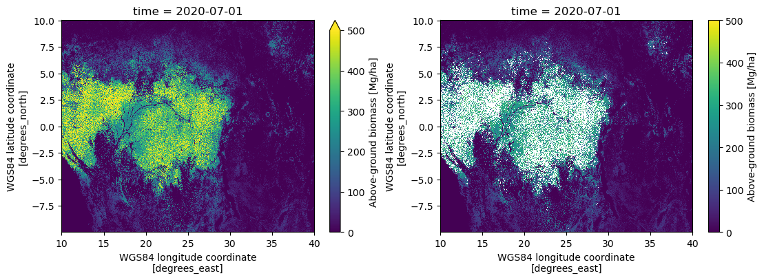
    tracking_id:                  cd5cb1d2-e582-41ab-a0fc-637f050baf9e

xarray.Dataset

• Dimensions:
  • time: 5
  • lat: 22500
  • lon: 33750
  • nv: 2
• Coordinates: (6)
  • lat
    (lat)
    float64
    10.0 9.999 9.998 ... -9.999 -10.0

    bounds :

    lat_bnds

    long_name :

    WGS84 latitude coordinate

    standard_name :

    latitude

    units :

    degrees_north

    valid_max :

    80.0

    valid_min :

    -60.0

    array([ 9.999556,  9.998667,  9.997778, ..., -9.997778, -9.998667, -9.999556])

  • lat_bnds
    (lat, nv)
    float64
    dask.array<chunksize=(1575, 2), meta=np.ndarray>

    Array Chunk Bytes 351.56 kiB 24.61 kiB Shape (22500, 2) (1575, 2) Dask graph 15 chunks in 3 graph layers Data type float64 numpy.ndarray

  • lon
    (lon)
    float64
    10.0 10.0 10.0 ... 40.0 40.0 40.0

    bounds :

    lon_bnds

    long_name :

    WGS84 longitude coordinate

    standard_name :

    longitude

    units :

    degrees_east

    valid_max :

    180.0

    valid_min :

    -180.0

    array([10.000444, 10.001333, 10.002222, ..., 39.997778, 39.998667, 39.999556])

  • lon_bnds
    (lon, nv)
    float64
    dask.array<chunksize=(900, 2), meta=np.ndarray>

    Array Chunk Bytes 527.34 kiB 31.64 kiB Shape (33750, 2) (2025, 2) Dask graph 18 chunks in 3 graph layers Data type float64 numpy.ndarray

  • time
    (time)
    datetime64[ns]
    2010-07-02 ... 2020-07-01

    array(['2010-07-02T00:00:00.000000000', '2017-07-02T00:00:00.000000000',
           '2018-07-02T00:00:00.000000000', '2019-07-02T00:00:00.000000000',
           '2020-07-01T00:00:00.000000000'], dtype='datetime64[ns]')

  • time_bnds
    (time, nv)
    datetime64[ns]
    dask.array<chunksize=(1, 2), meta=np.ndarray>

    Array Chunk Bytes 80 B 16 B Shape (5, 2) (1, 2) Dask graph 5 chunks in 2 graph layers Data type datetime64[ns] numpy.ndarray

• Data variables: (2)
  • agb
    (time, lat, lon)
    float32
    dask.array<chunksize=(1, 1575, 900), meta=np.ndarray>

    ancillary_variables :

    agb_se

    grid_mapping :

    crs

    long_name :

    Above-ground biomass

    units :

    Mg/ha

    valid_max :

    10000.0

    valid_min :

    0.0

    Array Chunk Bytes 14.14 GiB 12.17 MiB Shape (5, 22500, 33750) (1, 1575, 2025) Dask graph 1350 chunks in 3 graph layers Data type float32 numpy.ndarray

  • agb_se
    (time, lat, lon)
    float32
    dask.array<chunksize=(1, 1575, 900), meta=np.ndarray>

    grid_mapping :

    crs

    long_name :

    Above-ground biomass standard_error

    units :

    Mg/ha

    valid_max :

    10000.0

    valid_min :

    0.0

    Array Chunk Bytes 14.14 GiB 12.17 MiB Shape (5, 22500, 33750) (1, 1575, 2025) Dask graph 1350 chunks in 3 graph layers Data type float32 numpy.ndarray

• Indexes: (3)
  • lat
    PandasIndex

    PandasIndex(Index([ 9.999555556255558,  9.998666667366678,  9.997777778477797,
            9.996888889588917,  9.996000000700036,  9.995111111811156,
            9.994222222922275,  9.993333334033395,  9.992444445144514,
            9.991555556255634,
           ...
           -9.991555554655633, -9.992444443544514, -9.993333332433394,
           -9.994222221322275, -9.995111110211155, -9.995999999100036,
           -9.996888887988916, -9.997777776877797, -9.998666665766677,
           -9.999555554655558],
          dtype='float64', name='lat', length=22500))

  • lon
    PandasIndex

    PandasIndex(Index([10.000444442544449,  10.00133333143333,  10.00222222032221,
            10.00311110921109, 10.003999998099971, 10.004888886988851,
           10.005777775877732, 10.006666664766612, 10.007555553655465,
           10.008444442544345,
           ...
           39.991555553355624, 39.992444442244505, 39.993333331133385,
           39.994222220022266, 39.995111108911146,  39.99599999780003,
            39.99688888668891,  39.99777777557779,  39.99866666446667,
            39.99955555335555],
          dtype='float64', name='lon', length=33750))

  • time
    PandasIndex

    PandasIndex(DatetimeIndex(['2010-07-02', '2017-07-02', '2018-07-02', '2019-07-02',
                   '2020-07-01'],
                  dtype='datetime64[ns]', name='time', freq=None))

• Attributes: (53)

  Conventions :

  CF-1.7

  EPSG :

  4326

  GeoTransform :

  -180 0.00088888888888 0 80 0 -0.00088888888888

  catalogue_url :

  https://catalogue.ceda.ac.uk/uuid/84403d09cef3485883158f4df2989b0c

  cdm_data_type :

  INT

  comment :

  These data were produced at ESA CCI as part of the ESA Biomass CCI project.

  creator_email :

  santoro@gamma-rs.ch

  creator_name :

  GAMMA Remote Sensing

  creator_url :

  www.gamma-rs.ch

  date_created :

  21-Mar-2023 06:16:52

  false_easting :

  0.0

  false_northing :

  0.0

  format_version :

  CCI Data Standards v2.1

  geospatial_lat_max :

  80

  geospatial_lat_min :

  -60

  geospatial_lat_resolution :

  0.00088889

  geospatial_lat_units :

  degrees_north

  geospatial_lon_max :

  180

  geospatial_lon_min :

  -180

  geospatial_lon_resolution :

  0.00088889

  geospatial_lon_units :

  degrees_east

  geospatial_vertical_max :

  0.0

  geospatial_vertical_min :

  0.0

  grid_mapping_name :

  latitude_longitude

  history :

  AGB estimation with BIOMASAR-L, v202301, AGB estimation with BIOMASAR-C, v202301, Merging of AGB estimates, v202301

  id :

  ESACCI-BIOMASS-L4-AGB-MERGED-100m-2020-fv4.0.nc

  institution :

  GAMMA Remote Sensing

  inverse_flattening :

  298.257223563

  key_variables :

  agb

  keywords :

  satellite, observation, forest, biomass

  keywords_vocabulary :

  NASA Global Change Master Directory (GCMD) Science Keywords

  license :

  ESA CCI Data Policy: free and open access

  long_name :

  CRS definition

  longitude_of_prime_meridian :

  0.0

  naming authority :

  ch.gamma-rs

  platform :

  ALOS-2, Sentinel-1A, Sentinel-1B

  product_version :

  4.0

  proj4 :

  +proj=longlat +datum=WGS84 +no_defs

  project :

  Climate Change Initiative - European Space Agency

  references :

  http://cci.esa.int/biomass

  semi_major_axis :

  6378137.0

  sensor :

  PALSAR-2, SAR-C

  source :

  ALOS-2 PALSAR-2 FB and WB mosaics, Sentinel-1 GRD

  spatial_ref :

  GEOGCS["WGS 84",DATUM["WGS_1984",SPHEROID["WGS 84",6378137,298.257223563,AUTHORITY["EPSG","7030"]],AUTHORITY["EPSG","6326"]],PRIMEM["Greenwich",0],UNIT["degree",0.0174532925199433],AUTHORITY["EPSG","4326"]]

  spatial_resolution :

  100 m

  standard_name_vocabulary :

  NetCDF Climate and Forecast (CF) Metadata Convention version 67

  summary :

  This dataset contains a global map of above-ground biomass of the epoch 2020 obtained from L-and C-band spaceborne SAR backscatter, placed onto a regular grid.

  time_coverage_duration :

  P1Y

  time_coverage_end :

  20201231T000000Z

  time_coverage_resolution :

  P1Y

  time_coverage_start :

  20100101T000000Z

  title :

  ESA CCI above-ground biomass product level 4, year 2020

  tracking_id :

  cd5cb1d2-e582-41ab-a0fc-637f050baf9e

Where filter the dataset for standard error smaller than 100 Mg/ha.

filtered_ds = ds.where(ds["agb_se"] <= 100)
filtered_ds

<xarray.Dataset> Size: 30GB
Dimensions:    (time: 5, lat: 22500, lon: 33750, nv: 2)
Coordinates:
  * lat        (lat) float64 180kB 10.0 9.999 9.998 ... -9.998 -9.999 -10.0
    lat_bnds   (lat, nv) float64 360kB dask.array<chunksize=(1575, 2), meta=np.ndarray>
  * lon        (lon) float64 270kB 10.0 10.0 10.0 10.0 ... 40.0 40.0 40.0 40.0
    lon_bnds   (lon, nv) float64 540kB dask.array<chunksize=(900, 2), meta=np.ndarray>
  * time       (time) datetime64[ns] 40B 2010-07-02 2017-07-02 ... 2020-07-01
    time_bnds  (time, nv) datetime64[ns] 80B dask.array<chunksize=(1, 2), meta=np.ndarray>
Dimensions without coordinates: nv
Data variables:
    agb        (time, lat, lon) float32 15GB dask.array<chunksize=(1, 1575, 900), meta=np.ndarray>
    agb_se     (time, lat, lon) float32 15GB dask.array<chunksize=(1, 1575, 900), meta=np.ndarray>
Attributes: (12/53)
    Conventions:                  CF-1.7
    EPSG:                         4326
    GeoTransform:                 -180   0.00088888888888                  0 ...
    catalogue_url:                https://catalogue.ceda.ac.uk/uuid/84403d09c...
    cdm_data_type:                INT
    comment:                      These data were produced at ESA CCI as part...
    ...                           ...
    time_coverage_duration:       P1Y
    time_coverage_end:            20201231T000000Z
    time_coverage_resolution:     P1Y
    time_coverage_start:          20100101T000000Z
    title:                        ESA CCI above-ground biomass product level ...
    tracking_id:                  cd5cb1d2-e582-41ab-a0fc-637f050baf9e

xarray.Dataset

• Dimensions:
  • time: 5
  • lat: 22500
  • lon: 33750
  • nv: 2
• Coordinates: (6)
  • lat
    (lat)
    float64
    10.0 9.999 9.998 ... -9.999 -10.0

    bounds :

    lat_bnds

    long_name :

    WGS84 latitude coordinate

    standard_name :

    latitude

    units :

    degrees_north

    valid_max :

    80.0

    valid_min :

    -60.0

    array([ 9.999556,  9.998667,  9.997778, ..., -9.997778, -9.998667, -9.999556])

  • lat_bnds
    (lat, nv)
    float64
    dask.array<chunksize=(1575, 2), meta=np.ndarray>

    Array Chunk Bytes 351.56 kiB 24.61 kiB Shape (22500, 2) (1575, 2) Dask graph 15 chunks in 3 graph layers Data type float64 numpy.ndarray

  • lon
    (lon)
    float64
    10.0 10.0 10.0 ... 40.0 40.0 40.0

    bounds :

    lon_bnds

    long_name :

    WGS84 longitude coordinate

    standard_name :

    longitude

    units :

    degrees_east

    valid_max :

    180.0

    valid_min :

    -180.0

    array([10.000444, 10.001333, 10.002222, ..., 39.997778, 39.998667, 39.999556])

  • lon_bnds
    (lon, nv)
    float64
    dask.array<chunksize=(900, 2), meta=np.ndarray>

    Array Chunk Bytes 527.34 kiB 31.64 kiB Shape (33750, 2) (2025, 2) Dask graph 18 chunks in 3 graph layers Data type float64 numpy.ndarray

  • time
    (time)
    datetime64[ns]
    2010-07-02 ... 2020-07-01

    array(['2010-07-02T00:00:00.000000000', '2017-07-02T00:00:00.000000000',
           '2018-07-02T00:00:00.000000000', '2019-07-02T00:00:00.000000000',
           '2020-07-01T00:00:00.000000000'], dtype='datetime64[ns]')

  • time_bnds
    (time, nv)
    datetime64[ns]
    dask.array<chunksize=(1, 2), meta=np.ndarray>

    Array Chunk Bytes 80 B 16 B Shape (5, 2) (1, 2) Dask graph 5 chunks in 2 graph layers Data type datetime64[ns] numpy.ndarray

• Data variables: (2)
  • agb
    (time, lat, lon)
    float32
    dask.array<chunksize=(1, 1575, 900), meta=np.ndarray>

    ancillary_variables :

    agb_se

    grid_mapping :

    crs

    long_name :

    Above-ground biomass

    units :

    Mg/ha

    valid_max :

    10000.0

    valid_min :

    0.0

    Array Chunk Bytes 14.14 GiB 12.17 MiB Shape (5, 22500, 33750) (1, 1575, 2025) Dask graph 1350 chunks in 8 graph layers Data type float32 numpy.ndarray

  • agb_se
    (time, lat, lon)
    float32
    dask.array<chunksize=(1, 1575, 900), meta=np.ndarray>

    grid_mapping :

    crs

    long_name :

    Above-ground biomass standard_error

    units :

    Mg/ha

    valid_max :

    10000.0

    valid_min :

    0.0

    Array Chunk Bytes 14.14 GiB 12.17 MiB Shape (5, 22500, 33750) (1, 1575, 2025) Dask graph 1350 chunks in 5 graph layers Data type float32 numpy.ndarray

• Indexes: (3)
  • lat
    PandasIndex

    PandasIndex(Index([ 9.999555556255558,  9.998666667366678,  9.997777778477797,
            9.996888889588917,  9.996000000700036,  9.995111111811156,
            9.994222222922275,  9.993333334033395,  9.992444445144514,
            9.991555556255634,
           ...
           -9.991555554655633, -9.992444443544514, -9.993333332433394,
           -9.994222221322275, -9.995111110211155, -9.995999999100036,
           -9.996888887988916, -9.997777776877797, -9.998666665766677,
           -9.999555554655558],
          dtype='float64', name='lat', length=22500))

  • lon
    PandasIndex

    PandasIndex(Index([10.000444442544449,  10.00133333143333,  10.00222222032221,
            10.00311110921109, 10.003999998099971, 10.004888886988851,
           10.005777775877732, 10.006666664766612, 10.007555553655465,
           10.008444442544345,
           ...
           39.991555553355624, 39.992444442244505, 39.993333331133385,
           39.994222220022266, 39.995111108911146,  39.99599999780003,
            39.99688888668891,  39.99777777557779,  39.99866666446667,
            39.99955555335555],
          dtype='float64', name='lon', length=33750))

  • time
    PandasIndex

    PandasIndex(DatetimeIndex(['2010-07-02', '2017-07-02', '2018-07-02', '2019-07-02',
                   '2020-07-01'],
                  dtype='datetime64[ns]', name='time', freq=None))

• Attributes: (53)

  Conventions :

  CF-1.7

  EPSG :

  4326

  GeoTransform :

  -180 0.00088888888888 0 80 0 -0.00088888888888

  catalogue_url :

  https://catalogue.ceda.ac.uk/uuid/84403d09cef3485883158f4df2989b0c

  cdm_data_type :

  INT

  comment :

  These data were produced at ESA CCI as part of the ESA Biomass CCI project.

  creator_email :

  santoro@gamma-rs.ch

  creator_name :

  GAMMA Remote Sensing

  creator_url :

  www.gamma-rs.ch

  date_created :

  21-Mar-2023 06:16:52

  false_easting :

  0.0

  false_northing :

  0.0

  format_version :

  CCI Data Standards v2.1

  geospatial_lat_max :

  80

  geospatial_lat_min :

  -60

  geospatial_lat_resolution :

  0.00088889

  geospatial_lat_units :

  degrees_north

  geospatial_lon_max :

  180

  geospatial_lon_min :

  -180

  geospatial_lon_resolution :

  0.00088889

  geospatial_lon_units :

  degrees_east

  geospatial_vertical_max :

  0.0

  geospatial_vertical_min :

  0.0

  grid_mapping_name :

  latitude_longitude

  history :

  AGB estimation with BIOMASAR-L, v202301, AGB estimation with BIOMASAR-C, v202301, Merging of AGB estimates, v202301

  id :

  ESACCI-BIOMASS-L4-AGB-MERGED-100m-2020-fv4.0.nc

  institution :

  GAMMA Remote Sensing

  inverse_flattening :

  298.257223563

  key_variables :

  agb

  keywords :

  satellite, observation, forest, biomass

  keywords_vocabulary :

  NASA Global Change Master Directory (GCMD) Science Keywords

  license :

  ESA CCI Data Policy: free and open access

  long_name :

  CRS definition

  longitude_of_prime_meridian :

  0.0

  naming authority :

  ch.gamma-rs

  platform :

  ALOS-2, Sentinel-1A, Sentinel-1B

  product_version :

  4.0

  proj4 :

  +proj=longlat +datum=WGS84 +no_defs

  project :

  Climate Change Initiative - European Space Agency

  references :

  http://cci.esa.int/biomass

  semi_major_axis :

  6378137.0

  sensor :

  PALSAR-2, SAR-C

  source :

  ALOS-2 PALSAR-2 FB and WB mosaics, Sentinel-1 GRD

  spatial_ref :

  GEOGCS["WGS 84",DATUM["WGS_1984",SPHEROID["WGS 84",6378137,298.257223563,AUTHORITY["EPSG","7030"]],AUTHORITY["EPSG","6326"]],PRIMEM["Greenwich",0],UNIT["degree",0.0174532925199433],AUTHORITY["EPSG","4326"]]

  spatial_resolution :

  100 m

  standard_name_vocabulary :

  NetCDF Climate and Forecast (CF) Metadata Convention version 67

  summary :

  This dataset contains a global map of above-ground biomass of the epoch 2020 obtained from L-and C-band spaceborne SAR backscatter, placed onto a regular grid.

  time_coverage_duration :

  P1Y

  time_coverage_end :

  20201231T000000Z

  time_coverage_resolution :

  P1Y

  time_coverage_start :

  20100101T000000Z

  title :

  ESA CCI above-ground biomass product level 4, year 2020

  tracking_id :

  cd5cb1d2-e582-41ab-a0fc-637f050baf9e

We can generate a comparison plot that illustrates both the unfiltered and filtered above-ground biomass at a single time step as an example. Also here we downsample the dataset for the plotting.

fig, ax = plt.subplots(1, 2, figsize=(13, 4))
ds.agb.isel(time=-1)[::20, ::20].plot(ax=ax[0], vmin=0, vmax=500)
filtered_ds.agb.isel(time=-1)[::20, ::20].plot(ax=ax[1], vmin=0, vmax=500)

<matplotlib.collections.QuadMesh at 0x79ba646eec10>

---

4.2.2.4.3. 3. Filtering by any data feature

We will show this filtering operation on the soil moisture dataset, which also has other data variables which can be used for filtering.

ds = store.open_data("ESACCI-SOILMOISTURE-L3S-SSMV-COMBINED-1978-2021-fv07.1.zarr")
ds

<xarray.Dataset> Size: 654GB
Dimensions:         (time: 15767, lat: 720, lon: 1440)
Coordinates:
  * lat             (lat) float64 6kB 89.88 89.62 89.38 ... -89.38 -89.62 -89.88
  * lon             (lon) float64 12kB -179.9 -179.6 -179.4 ... 179.6 179.9
  * time            (time) datetime64[ns] 126kB 1978-11-01 ... 2021-12-31
Data variables:
    dnflag          (time, lat, lon) float32 65GB dask.array<chunksize=(16, 720, 720), meta=np.ndarray>
    flag            (time, lat, lon) float32 65GB dask.array<chunksize=(16, 720, 720), meta=np.ndarray>
    freqbandID      (time, lat, lon) float32 65GB dask.array<chunksize=(16, 720, 720), meta=np.ndarray>
    mode            (time, lat, lon) float32 65GB dask.array<chunksize=(16, 720, 720), meta=np.ndarray>
    sensor          (time, lat, lon) float64 131GB dask.array<chunksize=(16, 720, 720), meta=np.ndarray>
    sm              (time, lat, lon) float32 65GB dask.array<chunksize=(16, 720, 720), meta=np.ndarray>
    sm_uncertainty  (time, lat, lon) float32 65GB dask.array<chunksize=(16, 720, 720), meta=np.ndarray>
    t0              (time, lat, lon) float64 131GB dask.array<chunksize=(16, 720, 720), meta=np.ndarray>
Attributes: (12/44)
    Conventions:                  CF-1.9
    cdm_data_type:                Grid
    comment:                      This dataset was produced with funding of t...
    contact:                      cci_sm_contact@eodc.eu
    creator_email:                cci_sm_developer@eodc.eu
    creator_name:                 Department of Geodesy and Geoinformation, V...
    ...                           ...
    time_coverage_end_product:    20211231T235959Z
    time_coverage_resolution:     P1D
    time_coverage_start:          1978-11-01 00:00:00
    time_coverage_start_product:  19781101T000000Z
    title:                        ESA CCI Surface Soil Moisture COMBINED acti...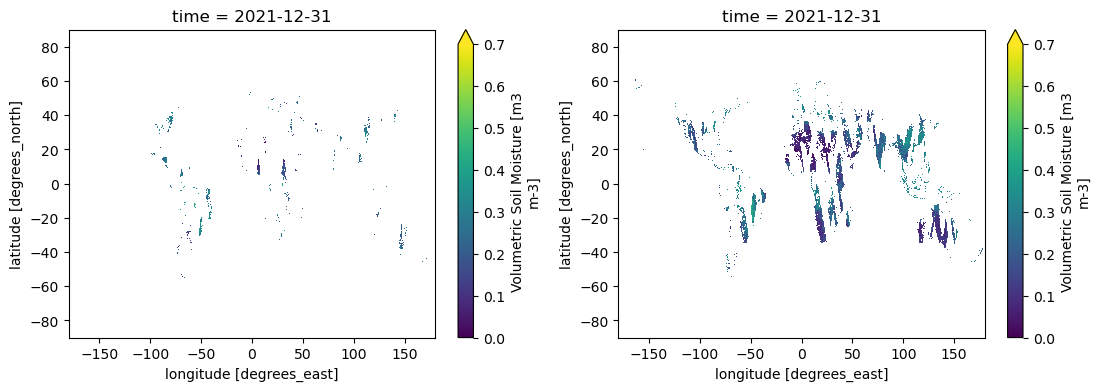
    tracking_id:                  ad35798e-58e0-488f-b5b9-593874a47700

xarray.Dataset

• Dimensions:
  • time: 15767
  • lat: 720
  • lon: 1440
• Coordinates: (3)
  • lat
    (lat)
    float64
    89.88 89.62 89.38 ... -89.62 -89.88

    _CoordinateAxisType :

    Lat

    standard_name :

    latitude

    units :

    degrees_north

    valid_range :

    [-90.0, 90.0]

    array([ 89.875,  89.625,  89.375, ..., -89.375, -89.625, -89.875])

  • lon
    (lon)
    float64
    -179.9 -179.6 ... 179.6 179.9

    _CoordinateAxisType :

    Lon

    standard_name :

    longitude

    units :

    degrees_east

    valid_range :

    [-180.0, 180.0]

    array([-179.875, -179.625, -179.375, ...,  179.375,  179.625,  179.875])

  • time
    (time)
    datetime64[ns]
    1978-11-01 ... 2021-12-31

    array(['1978-11-01T00:00:00.000000000', '1978-11-02T00:00:00.000000000',
           '1978-11-03T00:00:00.000000000', ..., '2021-12-29T00:00:00.000000000',
           '2021-12-30T00:00:00.000000000', '2021-12-31T00:00:00.000000000'],
          dtype='datetime64[ns]')

• Data variables: (8)
  • dnflag
    (time, lat, lon)
    float32
    dask.array<chunksize=(16, 720, 720), meta=np.ndarray>

    _CoordinateAxes :

    time lat lon

    bit_meanings :

    ['NaN', 'day', 'night']

    bits :

    ['0b0', '0b1', '0b10']

    dtype :

    int8

    flag_meanings :

    ['NaN', 'day', 'night', 'day_night_combination']

    flag_values :

    [0, 1, 2, 3]

    long_name :

    Day / Night Flag

    valid_range :

    [0, 3]

    Array Chunk Bytes 60.90 GiB 31.64 MiB Shape (15767, 720, 1440) (16, 720, 720) Dask graph 1972 chunks in 2 graph layers Data type float32 numpy.ndarray

  • flag
    (time, lat, lon)
    float32
    dask.array<chunksize=(16, 720, 720), meta=np.ndarray>

    _CoordinateAxes :

    time lat lon

    bit_meanings :

    ['no_data_inconsistency_detected', 'snow_coverage_or_temperature_below_zero', 'dense_vegetation', 'others_no_convergence_in_the_model_thus_no_valid_sm_estimates', 'soil_moisture_value_exceeds_physical_boundary', 'weight_of_measurement_below_threshold', 'all_datasets_deemed_unreliable', 'barren_ground_advisory_flag', 'NaN']

    bits :

    ['0b0', '0b1', '0b10', '0b100', '0b1000', '0b10000', '0b100000', '0b1000000', '0b10000000']

    dtype :

    int16

    flag_meanings :

    ['no_data_inconsistency_detected', 'snow_coverage_or_temperature_below_zero', 'dense_vegetation', 'combination_of_flag_values_1_and_2', 'soil_moisture_value_exceeds_physical_boundary', 'combination_of_flag_values_1_and_8', 'combination_of_flag_values_2_and_8', 'barren_ground_advisory_flag', 'combination_of_flag_values_1_and_64', 'combination_of_flag_values_2_and_64', 'combination_of_flag_values_1_and_2_and_64', 'combination_of_flag_values_8_and_64', 'combination_of_flag_values_1_and_8_and_64', 'combination_of_flag_values_2_and_8_and_64', 'combination_of_flag_values_1_and_2_and_4_and_8_and_16_and_32_and_64']

    flag_values :

    [0, 1, 2, 3, 8, 9, 10, 64, 65, 66, 67, 72, 73, 74, 127]

    long_name :

    Flag

    standard_name :

    soil_moisture_content status_flag

    valid_range :

    [0, 255]

    Array Chunk Bytes 60.90 GiB 31.64 MiB Shape (15767, 720, 1440) (16, 720, 720) Dask graph 1972 chunks in 2 graph layers Data type float32 numpy.ndarray

  • freqbandID
    (time, lat, lon)
    float32
    dask.array<chunksize=(16, 720, 720), meta=np.ndarray>

    _CoordinateAxes :

    time lat lon

    bit_meanings :

    ['NaN', 'L14', 'C53', 'C66', 'C68', 'C69', 'C73', 'X107', 'K194', 'MODEL']

    bits :

    ['0b0', '0b1', '0b10', '0b100', '0b1000', '0b10000', '0b100000', '0b1000000', '0b10000000', '0b100000000']

    dtype :

    int16

    flag_meanings :

    ['NaN', 'C66', 'X107', 'C66+X107']

    flag_values :

    [0, 4, 64, 68]

    long_name :

    Frequency Band Identification

    valid_range :

    [0, 511]

    Array Chunk Bytes 60.90 GiB 31.64 MiB Shape (15767, 720, 1440) (16, 720, 720) Dask graph 1972 chunks in 2 graph layers Data type float32 numpy.ndarray

  • mode
    (time, lat, lon)
    float32
    dask.array<chunksize=(16, 720, 720), meta=np.ndarray>

    _CoordinateAxes :

    time lat lon

    bit_meanings :

    ['NaN', 'ascending', 'descending']

    bits :

    ['0b0', '0b1', '0b10']

    dtype :

    int8

    flag_meanings :

    ['NaN', 'ascending', 'descending', 'ascending_descending_combination']

    flag_values :

    [0, 1, 2, 3]

    long_name :

    Satellite Mode

    valid_range :

    [0, 3]

    Array Chunk Bytes 60.90 GiB 31.64 MiB Shape (15767, 720, 1440) (16, 720, 720) Dask graph 1972 chunks in 2 graph layers Data type float32 numpy.ndarray

  • sensor
    (time, lat, lon)
    float64
    dask.array<chunksize=(16, 720, 720), meta=np.ndarray>

    _CoordinateAxes :

    time lat lon

    bit_meanings :

    ['NaN', 'SMMR', 'SSMI', 'TMI', 'AMSRE', 'WindSat', 'AMSR2', 'SMOS', 'AMIWS', 'ASCATA', 'ASCATB', 'SMAP', 'MODEL', 'GPM', 'FY3B', 'FY3D', 'ASCATC', 'FY3C']

    bits :

    ['0b0', '0b1', '0b10', '0b100', '0b1000', '0b10000', '0b100000', '0b1000000', '0b10000000', '0b100000000', '0b1000000000', '0b10000000000', '0b100000000000', '0b1000000000000', '0b10000000000000', '0b100000000000000', '0b1000000000000000', '0b10000000000000000']

    dtype :

    int32

    flag_meanings :

    ['NaN', 'SMMR']

    flag_values :

    [0, 1]

    long_name :

    Sensor

    valid_range :

    [0, 131071]

    Array Chunk Bytes 121.80 GiB 63.28 MiB Shape (15767, 720, 1440) (16, 720, 720) Dask graph 1972 chunks in 2 graph layers Data type float64 numpy.ndarray

  • sm
    (time, lat, lon)
    float32
    dask.array<chunksize=(16, 720, 720), meta=np.ndarray>

    _CoordinateAxes :

    time lat lon

    ancillary_variables :

    sm_uncertainty flag t0

    dtype :

    float32

    long_name :

    Volumetric Soil Moisture

    standard_name :

    soil_moisture_content

    units :

    m3 m-3

    valid_range :

    [0.0, 1.0]

    Array Chunk Bytes 60.90 GiB 31.64 MiB Shape (15767, 720, 1440) (16, 720, 720) Dask graph 1972 chunks in 2 graph layers Data type float32 numpy.ndarray

  • sm_uncertainty
    (time, lat, lon)
    float32
    dask.array<chunksize=(16, 720, 720), meta=np.ndarray>

    _CoordinateAxes :

    time lat lon

    dtype :

    float32

    long_name :

    Volumetric Soil Moisture Uncertainty

    standard_name :

    soil_moisture_content standard_error

    units :

    m3 m-3

    valid_range :

    [0.0, 1.0]

    Array Chunk Bytes 60.90 GiB 31.64 MiB Shape (15767, 720, 1440) (16, 720, 720) Dask graph 1972 chunks in 2 graph layers Data type float32 numpy.ndarray

  • t0
    (time, lat, lon)
    float64
    dask.array<chunksize=(16, 720, 720), meta=np.ndarray>

    _CoordinateAxes :

    time lat lon

    dtype :

    float64

    long_name :

    Observation Timestamp

    units :

    days after 1970-01-01 00:00:00 UTC

    valid_range :

    [3225.0, 3227.0]

    Array Chunk Bytes 121.80 GiB 63.28 MiB Shape (15767, 720, 1440) (16, 720, 720) Dask graph 1972 chunks in 2 graph layers Data type float64 numpy.ndarray

• Indexes: (3)
  • lat
    PandasIndex

    PandasIndex(Index([ 89.875,  89.625,  89.375,  89.125,  88.875,  88.625,  88.375,  88.125,
            87.875,  87.625,
           ...
           -87.625, -87.875, -88.125, -88.375, -88.625, -88.875, -89.125, -89.375,
           -89.625, -89.875],
          dtype='float64', name='lat', length=720))

  • lon
    PandasIndex

    PandasIndex(Index([-179.875, -179.625, -179.375, -179.125, -178.875, -178.625, -178.375,
           -178.125, -177.875, -177.625,
           ...
            177.625,  177.875,  178.125,  178.375,  178.625,  178.875,  179.125,
            179.375,  179.625,  179.875],
          dtype='float64', name='lon', length=1440))

  • time
    PandasIndex

    PandasIndex(DatetimeIndex(['1978-11-01', '1978-11-02', '1978-11-03', '1978-11-04',
                   '1978-11-05', '1978-11-06', '1978-11-07', '1978-11-08',
                   '1978-11-09', '1978-11-10',
                   ...
                   '2021-12-22', '2021-12-23', '2021-12-24', '2021-12-25',
                   '2021-12-26', '2021-12-27', '2021-12-28', '2021-12-29',
                   '2021-12-30', '2021-12-31'],
                  dtype='datetime64[ns]', name='time', length=15767, freq=None))

• Attributes: (44)

  Conventions :

  CF-1.9

  cdm_data_type :

  Grid

  comment :

  This dataset was produced with funding of the ESA CCI+ Soil Moisture project; ESRIN Contract No: 4000126684/19/I-NB

  contact :

  cci_sm_contact@eodc.eu

  creator_email :

  cci_sm_developer@eodc.eu

  creator_name :

  Department of Geodesy and Geoinformation, Vienna University of Technology

  creator_url :

  https://climers.geo.tuwien.ac.at/

  date_created :

  File created: 2022-04-06 12:31:39.526359

  geospatial_lat_max :

  90.0

  geospatial_lat_min :

  -90.0

  geospatial_lat_resolution :

  0.25 degree

  geospatial_lat_units :

  degrees_north

  geospatial_lon_max :

  180.0

  geospatial_lon_min :

  -180.0

  geospatial_lon_resolution :

  0.25 degree

  geospatial_lon_units :

  degrees_east

  geospatial_vertical_max :

  0.0

  geospatial_vertical_min :

  0.0

  history :

  2022-04-06 12:29:35 - product produced 2023-08-09 17:33:51 - converted by nc2zarr, version 1.1.2.dev0

  id :

  ESACCI-SOILMOISTURE-L3S-SSMV-COMBINED-20211231000000-fv07.1.nc

  institution :

  TU Wien (AUT); VanderSat B.V. (NL)

  key_variables :

  sm

  keywords :

  soil moisture, soil water content, microwave remote sensing, active, passive, combined, climate data record

  keywords_vocabulary :

  NASA Global Change Master Directory (GCMD) Science Keywords

  license :

  Data use is free and open for all registered users.

  naming_authority :

  TU Wien

  platform :

  Nimbus 7, DMSP, TRMM, AQUA, Coriolis, GCOM-W1, MIRAS, SMAP, GPM, FengYun-3B, FengYun-3C, FengYun-3D; ERS-1, ERS-2, METOP-A, METOP-B

  processing_level :

  Quality-controlled, super-collocated (L3S) Satellite Soil Moisture (SM) data from multiple sensors

  product_version :

  v07.1

  project :

  Climate Change Initiative - European Space Agency

  references :

  http://www.esa-soilmoisture-cci.org; Dorigo, W.A., Wagner, W., Albergel, C., Albrecht, F., Balsamo, G., Brocca, L., Chung, D., Ertl, M., Forkel, M., Gruber, A., Haas, E., Hamer, D. P. Hirschi, M., Ikonen, J., De Jeu, R. Kidd, R. Lahoz, W., Liu, Y.Y., Miralles, D., Lecomte, P. (2017) ESA CCI Soil Moisture for improved Earth system understanding: State-of-the art and future directions. In Remote Sensing of Environment, 2017, ISSN 0034-4257, https://doi.org/10.1016/j.rse.2017.07.001; Gruber, A., Scanlon, T., van der Schalie, R., Wagner, W., Dorigo, W. (2019) Evolution of the ESA CCI Soil Moisture Climate Data Records and their underlying merging methodology. Earth System Science Data 11, 717-739, https://doi.org/10.5194/essd-11-717-2019; Gruber, A., Dorigo, W. A., Crow, W., Wagner W. (2017). Triple Collocation-Based Merging of Satellite Soil Moisture Retrievals. IEEE Transactions on Geoscience and Remote Sensing. PP. 1-13. https://doi.org/10.1109/TGRS.2017.2734070

  sensor :

  SMMR, SSM/I, TMI, AMSR-E, WindSat, AMSR2, SMOS, SMAP_radiometer, GMI, VIRR-3B, VIRR-3C, VIRR-3D; AMI-WS, ASCAT-A, ASCAT-B, ASCAT-C

  source :

  WARP 5.5R1.1/AMI-WS/ERS12 Level 2 Soil Moisture; WARP 5.4R1.0/AMI-WS/ERS2 Level 2 Soil Moisture; H115: Metop ASCAT Surface Soil Moisture Climate Data Record v5 12.5 km sampling, DOI: 10.15770/EUM_SAF_H_0006; H116: Metop ASCAT Surface Soil Moisture Climate Data Record v5 Extension 12.5 km sampling; H115: Metop ASCAT Surface Soil Moisture Climate Data Record v5 12.5 km sampling, DOI: 10.15770/EUM_SAF_H_0006; H116: Metop ASCAT Surface Soil Moisture Climate Data Record v5 Extension 12.5 km sampling; H115: Metop ASCAT Surface Soil Moisture Climate Data Record v5 12.5 km sampling, DOI: 10.15770/EUM_SAF_H_0006; H116: Metop ASCAT Surface Soil Moisture Climate Data Record v5 Extension 12.5 km sampling;; LPRMv7/SMMR/Nimbus 7 L3 Surface Soil Moisture, Ancillary Params, and quality flags; LPRMv7/SSMI/F08, F11, F13 DMSP L3 Surface Soil Moisture, Ancillary Params, and quality flags; LPRMv7/TMI/TRMM L2 Surface Soil Moisture, Ancillary Params, and QC; LPRMv7/AMSR-E/Aqua L2B Surface Soil Moisture, Ancillary Params, and QC; LPRMv7/WINDSAT/CORIOLIS L2 Surface Soil Moisture, Ancillary Params, and QC; LPRMv7/AMSR2/GCOM-W1 L3 Surface Soil Moisture, Ancillary Params; LPRMv7/SMOS/MIRAS L3 Surface Soil Moisture, CATDS Level 3 Brightness Temperatures (L3TB) version 300 RE03 & RE04; LPRMv7/SMAP_radiometer/SMAP L2 Surface Soil Moisture, Ancillary Params, and QC; LPRMv7/GMI/GPM L3 Surface Soil Moisture, Ancillary Params, and quality flags; LPRMv7/VIRR/FengYun-3B L3 Surface Soil Moisture, Ancillary Params, and quality flags; LPRMv7/VIRR/FengYun-3C L3 Surface Soil Moisture, Ancillary Params, and quality flags; LPRMv7/VIRR/FengYun-3D L3 Surface Soil Moisture, Ancillary Params, and quality flags;;

  spatial_resolution :

  25km

  standard_name_vocabulary :

  CF Standard Name Table v77

  summary :

  This dataset was produced with funding of the ESA CCI+ Soil Moisture project; ESRIN Contract No: 4000126684/19/I-NB

  time_coverage_duration :

  P43Y

  time_coverage_end :

  2021-12-31 00:00:00

  time_coverage_end_product :

  20211231T235959Z

  time_coverage_resolution :

  P1D

  time_coverage_start :

  1978-11-01 00:00:00

  time_coverage_start_product :

  19781101T000000Z

  title :

  ESA CCI Surface Soil Moisture COMBINED active+passive Product

  tracking_id :

  ad35798e-58e0-488f-b5b9-593874a47700

For example, we can use the data variable "mode", which indicates whether the observation is derived from the ascending or descending orbit. This variable can be used to filter the dataset, allowing us to select only the ascending mode, represented by 1, and the descending mode, represented by 2, and as shown below:

fig, ax = plt.subplots(1, 2, figsize=(13, 4))
ds.where(ds["mode"] == 1).sm.isel(time=-1).plot(ax=ax[0], vmin=0, vmax=0.7)
ds.where(ds["mode"] == 2).sm.isel(time=-1).plot(ax=ax[1], vmin=0, vmax=0.7)

<matplotlib.collections.QuadMesh at 0x79ba535e34d0>

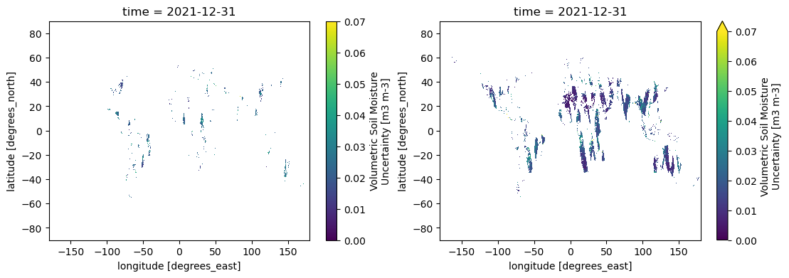
We can easliy generate the same plot for the soil moisture uncertainty data variable.

fig, ax = plt.subplots(1, 2, figsize=(13, 4))
ds.where(ds["mode"] == 1).sm_uncertainty.isel(time=-1).plot(ax=ax[0], vmin=0, vmax=0.07)
ds.where(ds["mode"] == 2).sm_uncertainty.isel(time=-1).plot(ax=ax[1], vmin=0, vmax=0.07)

<matplotlib.collections.QuadMesh at 0x79ba643c42d0>